Supporting material for the article:
Adaptive Sample Size and Importance Sampling in
Estimation-based Local Search
for the Probabilistic Traveling Salesman Problem
April 2008
1. Abstract:
The probabilistic traveling salesman problem is a paradigmatic example of a stochastic combinatorial optimization problem. For this problem, recently, an estimation-based local search algorithm using delta evaluation has been proposed. In this paper, we adopt two well-known variance reduction procedures in the estimation-based local search algorithm: The first is an adaptive sampling procedure that selects the appropriate size of the sample to be used in Monte Carlo evaluation; the second is a procedure that adopts the importance sampling technique. We investigate several possible strategies of applying these procedures for the given problem and we identify the most effective one. Experimental results show that a particular problem specific customization of the two procedures increases significantly the effectiveness of the estimation-based local search.
Keywords: Probabilistic Traveling Salesman Problem, Local Search, Iterative Improvement Algorithm, Empirical Estimation, Delta Evaluation, Adaptive Sample Size, Importance Sampling
2. Algorithms:
- 2-p-opt and 1-shift: The state-of-the-art iterative improvement algorithms for PTSP
- 2.5-opt-ACs: 2.5-opt neighborhood exploration and neighborhood reduction techniques(fixed-radius search, candidate lists and don’t look bits) in the analytical computation framework.
- 2.5-opt-EEs: 2.5-opt neighborhood exploration and neighborhood reduction techniques(fixed-radius search, candidate lists and don’t look bits) in the empirical estimation framework.
- 2.5-opt-EEs-10: 2.5-opt-EEs with 10 realizations
- 2.5-opt-EEs-100: 2.5-opt-EEs with 100 realizations
- 2.5-opt-EEs-1000: 2.5-opt-EEs with 1000 realizations
- 2.5-opt-EEas: 2.5-opt-EEs with adaptive sample size.
- 2.5-opt-EEais: 2.5-opt-EEs with adaptive sample size and importance sampling technique.
- ILS-2.5-opt-ACs: Iterated local search with 2.5-opt-ACs.
- ILS-2.5-opt-EEais: Iterated local search with 2.5-opt-EEais.
3. Experiments on neighborhood-reduction techniques
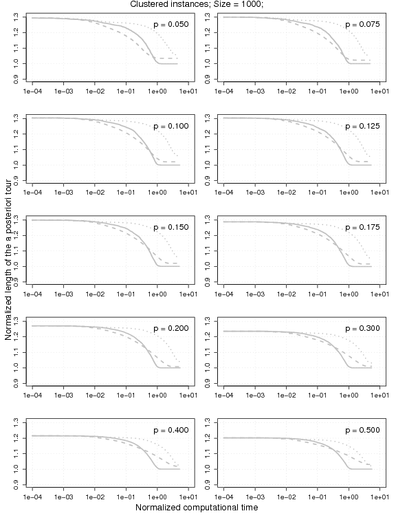
Experimental results on
clustered homogeneous PTSP instances of size 1000 (1.1 MB). The plots represent the average cost of the solutions obtained by
2-p-opt and
1-shift normalized by the one obtained by
2.5-opt-ACs. Each algorithm is stopped when it reaches a local optimum.
 |
 |
4. Instances used for tuning :
We tuned each importance sampling variant separately for the homogenous and the heterogeneous clustered instances of size 1000. We used 210 instances (7 levels of probability and 30 instances for each level) for the homogeneous case and 210 instances (7 levels of probability and 3 levels of percentage of maximum variance and 10 instances each) for the heterogeneous case.
5. A study on the parameters of ILS-2.5-opt-EEais
5.1 Importance sampling variants
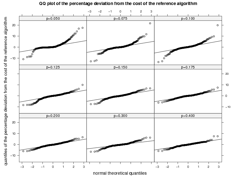
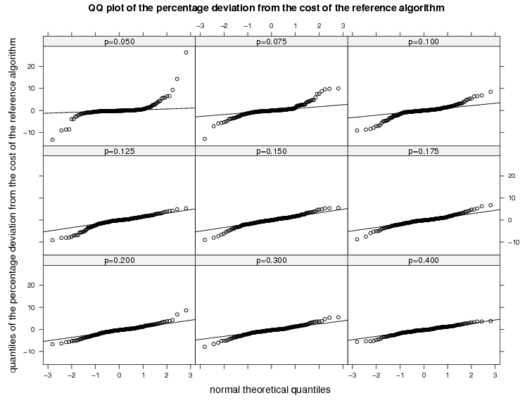
QQ plot to test the normality of the cost of 2.5-opt-EEais as the percentage deviation from the cost of 2.5-opt-EEs-1000 for different importance sampling variants: uniform biasing (ub), geometric biasing (gb), strong greedy biasing (sb), weak greedy (wb), and problem-specific biasing (pb) (homogeneous instances of size 1000).
 |
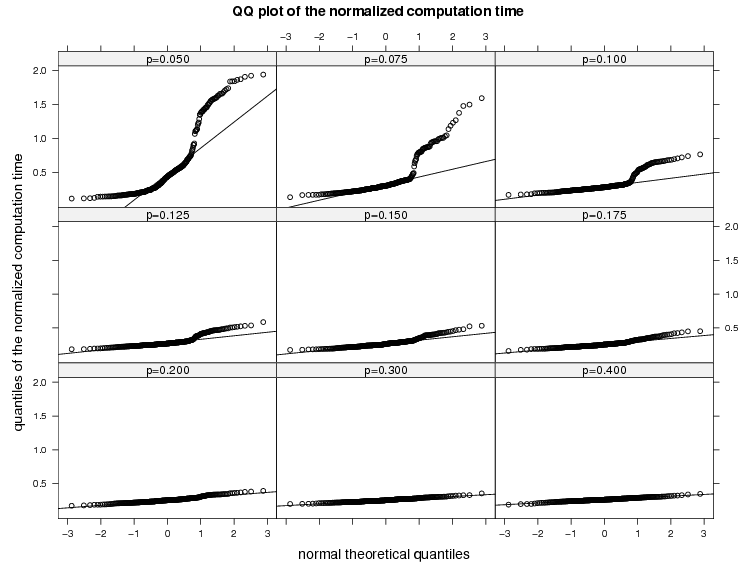
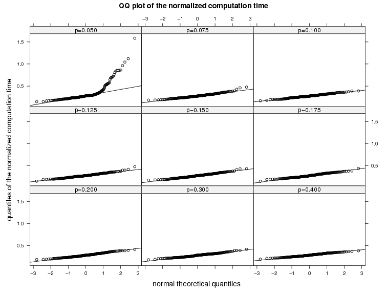
< align="left">QQ plot to test the normality of the the normalized computation time of 2.5-opt-EEais where the normalization is done with respect to the computation time of 2.5-opt-EEs-1000 for different importance sampling variants: uniform biasing (ub), geometric biasing (gb), strong greedy biasing (sb), weak greedy (wb), and problem-specific biasing (pb) (homogeneous instances of size 1000).
 |
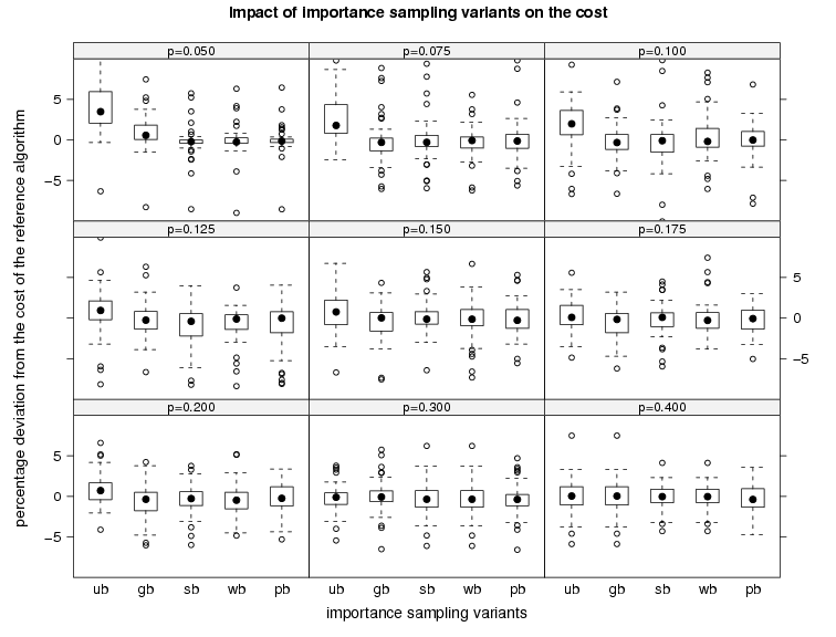
The plot shows the cost of the solutions of 2.5-opt-EEais as the percentage deviation from the cost of 2.5-opt-EE-1000 for different importance sampling variants: uniform biasing (ub), geometric biasing (gb), strong greedy biasing (sb), weak greedy (wb), and problem-specific biasing (pb) (homogeneous instances of size 1000).
 |
| ANOVA summary |
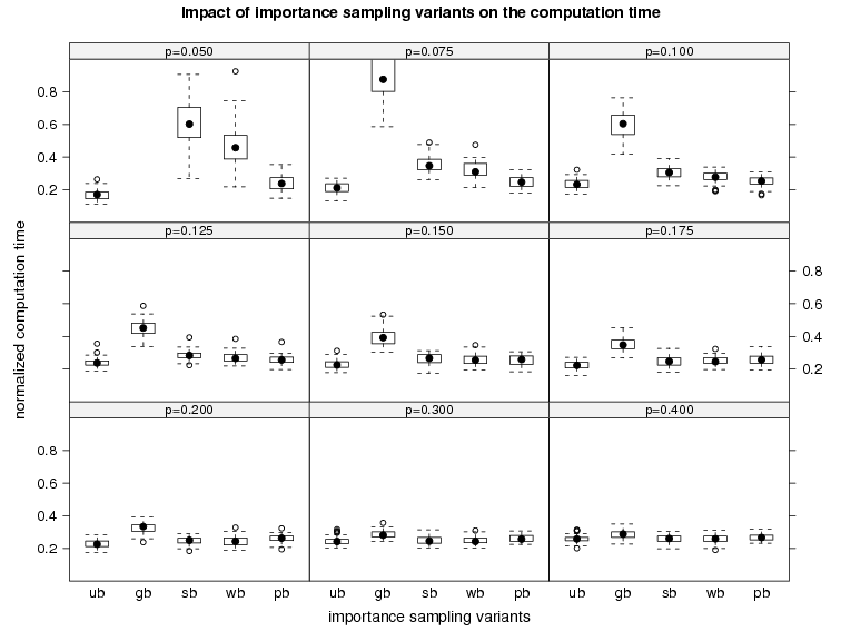
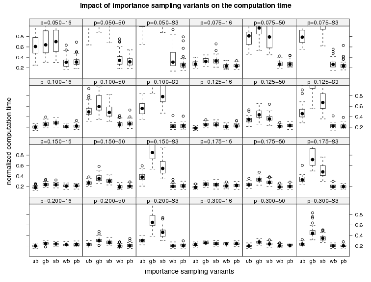
The plot shows the normalized computation time of 2.5-opt-EEais where the normalization is done with respect to the computation time of 2.5-opt-EEs-1000 for for different importance sampling variants: uniform biasing (ub), geometric biasing (gb), strong greedy biasing (sb), weak greedy (wb), and problem-specific biasing (pb) (homogeneous instances of size 1000).
 |
| ANOVA summary |
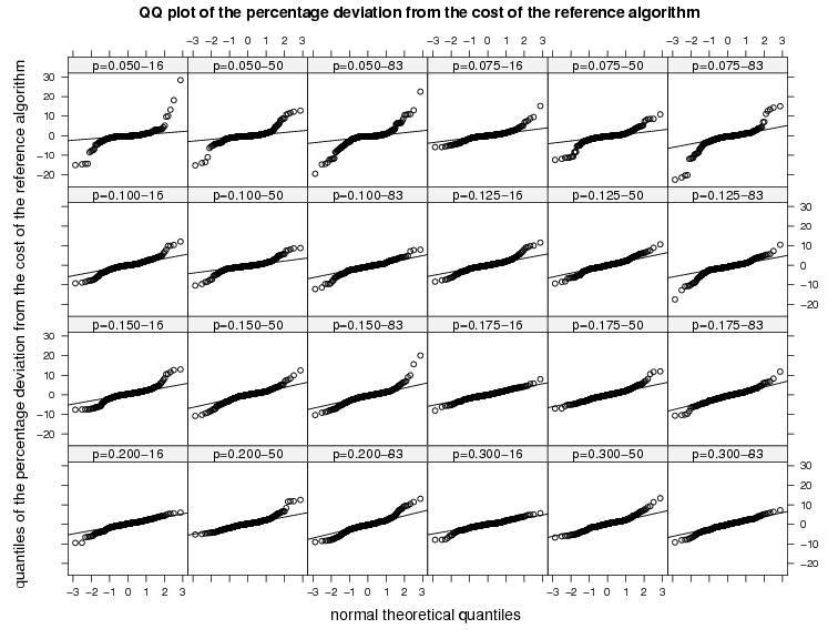
QQ plot to test the normality of the cost of 2.5-opt-EEais as the percentage deviation from the cost of 2.5-opt-EEs-1000 for different importance sampling variants: uniform biasing (ub), geometric biasing (gb), strong greedy biasing (sb), weak greedy (wb), and problem-specific biasing (pb) (heterogeneous instances of size 1000).
 |
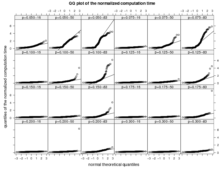
QQ plot to test the normality of the the normalized computation time of 2.5-opt-EEais where the normalization is done with respect to the computation time of 2.5-opt-EEs-1000 for different importance sampling variants: uniform biasing (ub), geometric biasing (gb), strong greedy biasing (sb), weak greedy (wb), and problem-specific biasing (pb) (heterogeneous instances of size 1000).
 |
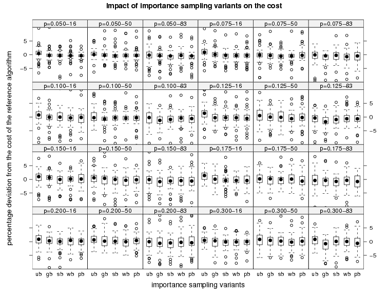
The plot shows the cost of the solutions of 2.5-opt-EEais as the percentage deviation from the cost of 2.5-opt-EE-1000 for different importance sampling variants: uniform biasing (ub), geometric biasing (gb), strong greedy biasing (sb), weak greedy (wb), and problem-specific biasing (pb) (eterogeneous instances of size 1000).
 |
| ANOVA summary |
The plot shows the normalized computation time of 2.5-opt-EEais where the normalization is done with respect to the computation time of 2.5-opt-EEs-1000 for for different importance sampling variants: uniform biasing (ub), geometric biasing (gb), strong greedy biasing (sb), weak greedy (wb), and problem-specific biasing (pb) (eterogeneous instances of size 1000).
 |
| ANOVA summary |
5.2 Significance level
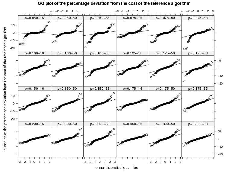
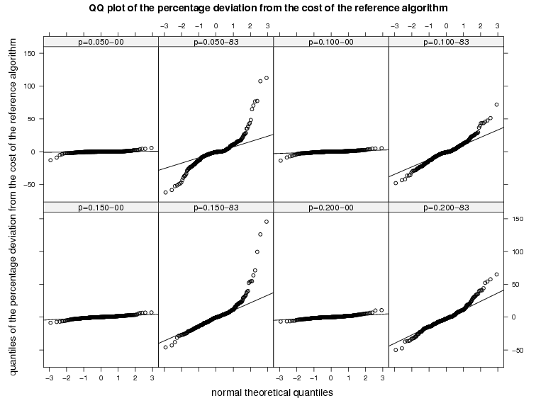
QQ plot to test the normality of the cost of 2.5-opt-EEais with problem-specific biasing as the percentage deviation from the cost of 2.5-opt-EEs-1000 for different significance levels (homogeneous instances of size 1000).
 |
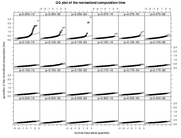
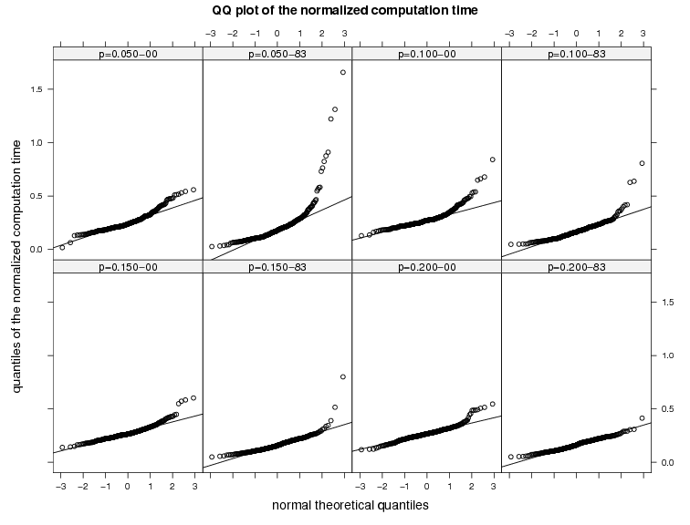
QQ plot to test the normality of the the normalized computation time of 2.5-opt-EEais with problem-specific biasing (pb), where the normalization is done with respect to the computation time of 2.5-opt-EEs-1000 for different significance levels (homogeneous instances of size 1000).
 |
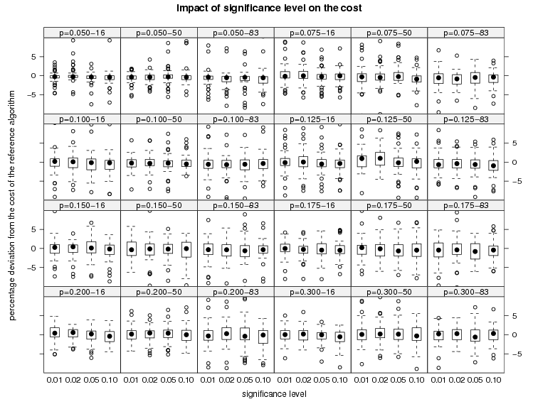
The plot shows the cost of the solutions of 2.5-opt-EEais with problem-specific biasing as the percentage deviation from the cost of 2.5-opt-EE-1000 for different significance levels (homogeneous instances of size 1000).
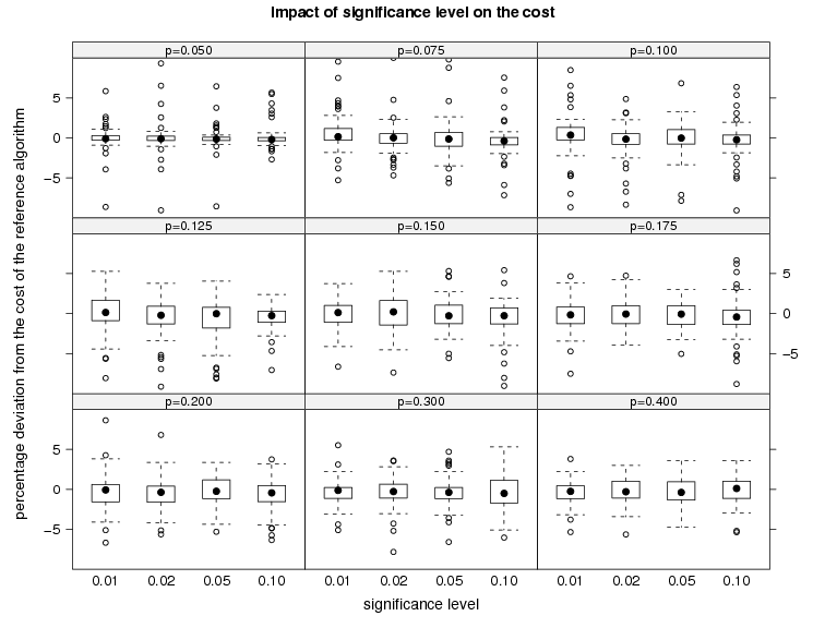 |
| ANOVA summary |
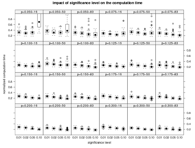
The plot shows the normalized computation time of 2.5-opt-EEais with problem-specific biasing where the normalization is done with respect to the computation time of 2.5-opt-EEs-1000 for for different significance levels (homogeneous instances of size 1000).
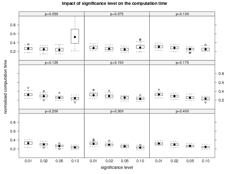 |
| ANOVA summary |
QQ plot to test the normality of the cost of 2.5-opt-EEais with problem-specific biasing as the percentage deviation from the cost of 2.5-opt-EEs-1000 for different significance levels (heterogeneous instances of size 1000).
 |
QQ plot to test the normality of the the normalized computation time of 2.5-opt-EEais with problem-specific biasing (pb), where the normalization is done with respect to the computation time of 2.5-opt-EEs-1000 for different significance levels (heterogeneous instances of size 1000).
 |
The plot shows the cost of the solutions of 2.5-opt-EEais with problem-specific biasing as the percentage deviation from the cost of 2.5-opt-EE-1000 for different significance levels (heterogeneous instances of size 1000).
 |
| ANOVA summary |
The plot shows the normalized computation time of 2.5-opt-EEais with problem-specific biasing where the normalization is done with respect to the computation time of 2.5-opt-EEs-1000 for different significance levels (heterogeneous instances of size 1000).
 |
| ANOVA summary |
5.3 Instance size and distribution of nodes
QQ plot to test the normality of the cost of 2.5-opt-EEais with problem-specific biasing (pb) as the percentage deviation from the cost of 2.5-opt-EEs-1000.
 |
QQ plot to test the normality of the the normalized computation time of 2.5-opt-EEais with problem-specific biasing (pb), where the normalization is done with respect to the computation time of 2.5-opt-EEs-1000.
 |
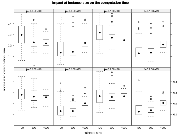
The plot shows the cost of the solutions of 2.5-opt-EEais with problem-specific biasing as the percentage deviation from the cost of 2.5-opt-EE-1000 for different instance sizes.
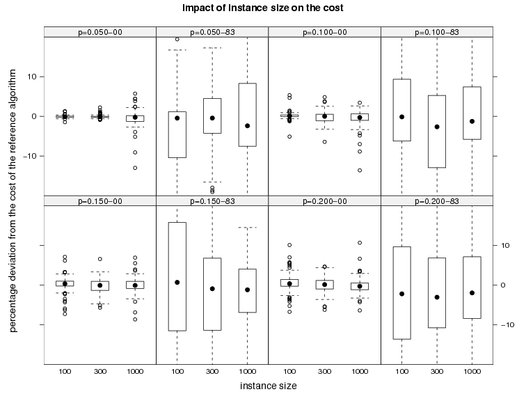 |
The plot shows the normalized computation time of 2.5-opt-EEais with problem-specific biasing where the normalization is done with respect to the computation time of 2.5-opt-EEs-1000 for different instance sizes.
 |
| ANOVA summary |
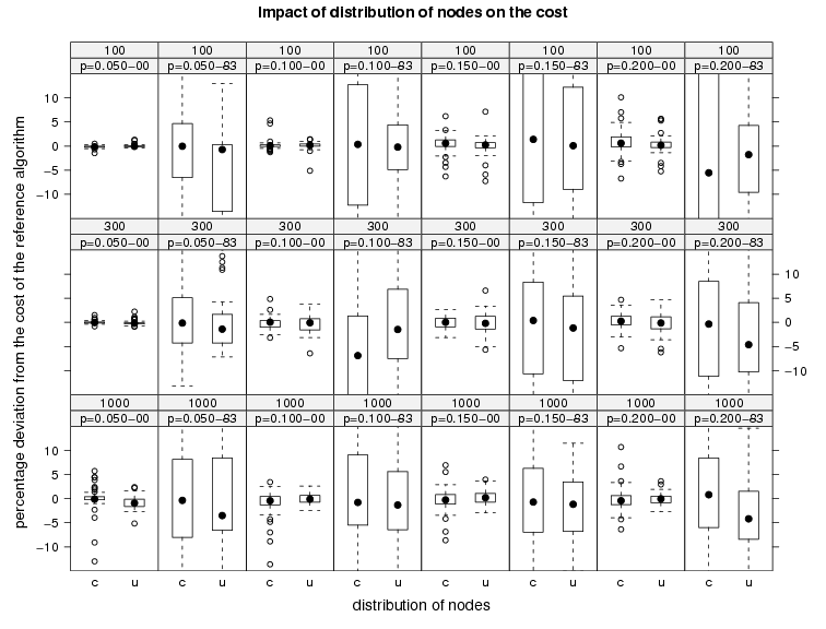
The plot shows the cost of the solutions of 2.5-opt-EEais with problem-specific biasing as the percentage deviation from the cost of 2.5-opt-EE-1000 for clustered (c) and uniform (u) instances.
 |
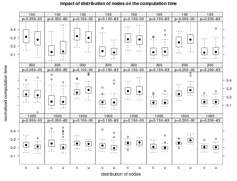
The plot shows the normalized computation time of 2.5-opt-EEais with problem-specific biasing where the normalization is done with respect to the computation time of 2.5-opt-EEs-1000 for clustered (c) and uniform (u) instances.
 |
| ANOVA summary |
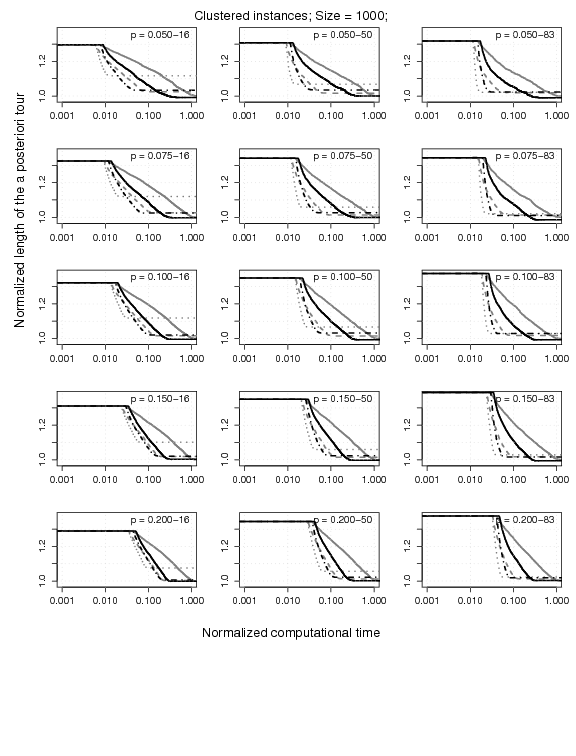
6. Experiments with estimation-based algorithms
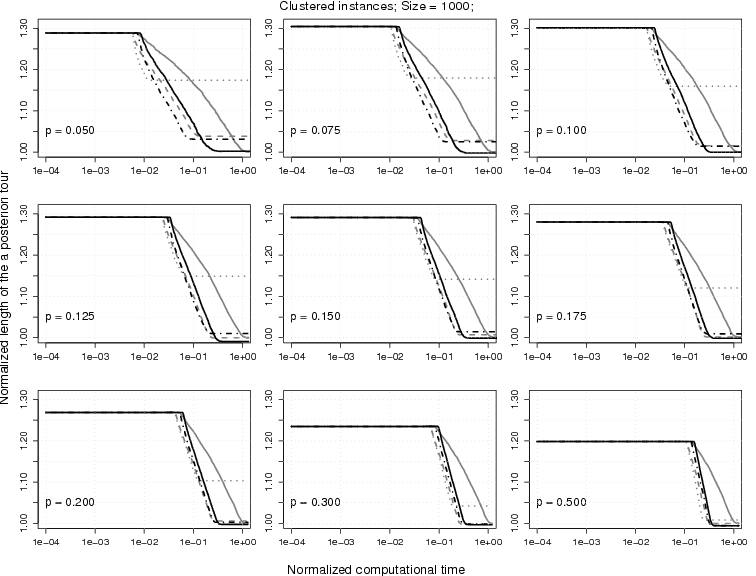
Experimental results on
clustered homogeneous PTSP instances of size 1000 (1.9 MB). The plots represent the cost of the solutions obtained by 2.5-opt-EEais, 2.5-opt-EEas, 2.5-opt-EE-10, and 2.5-opt-EE-100 normalized by the one obtained by 2.5-opt-EE-1000. Each algorithm is stopped when it reaches a local optimum. The normalization is done on an instance by instance basis for 50 instances; the normalized solution cost and the computation time are then aggregated. Note that the x-axis shows the computation time in logarithmic scale.
 |
 |
Experimental results on
clustered heterogeneous PTSP instances of size 1000(9 MB). The plots represent the cost of the solutions obtained by 2.5-opt-EEais, 2.5-opt-EEas, 2.5-opt-EE-10, and 2.5-opt-EE-100 normalized by the one obtained by 2.5-opt-EE-1000. Each algorithm is stopped when it reaches a local optimum. The normalization is done on an instance by instance basis for 50 instances; the normalized solution cost and the computation time are then aggregated. Note that the x-axis shows the computation time in logarithmic scale.
 |
|
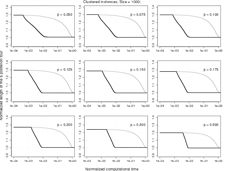
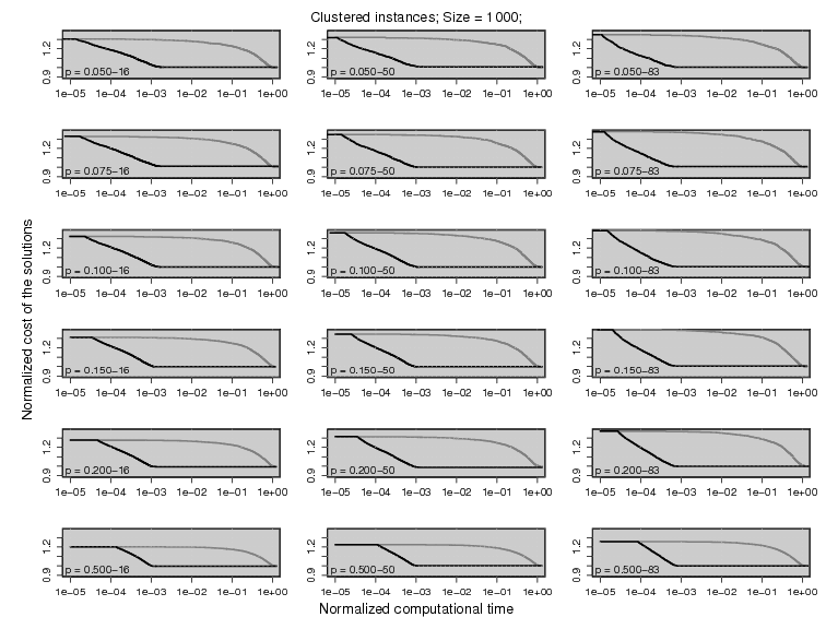
7. Experiments with the analytical computation algorithms
Experimental results on
clustered homogeneous PTSP instances of size 1000 (1.9 MB). The plots represent the cost of the solutions obtained by 2.5-opt-EEais normalized by the one obtained by 2.5-opt-ACs. Each algorithm is stopped when it reaches a local optimum. The normalization is done on an instance by instance basis for 50 instances; the normalized solution cost and the computation time are then aggregated. Note that the x-axis shows the computation time in logarithmic scale.
 |
 |
Experimental results on
clustered heterogeneous PTSP instances of size 1000 (9 MB). The plots represent the cost of the solutions obtained by 2.5-opt-EEais normalized by the one obtained by 2.5-opt-ACs. Each algorithm is stopped when it reaches a local optimum. 2.5-opt-ACs use a library for arbitrary precision arithmetics. To emphasize this fact the backgrounds of plots are gray. The normalization is done on an instance by instance basis for 50 instances; the normalized solution cost and the computation time are then aggregated. Note that the x-axis shows the computation time in logarithmic scale.
 |
|
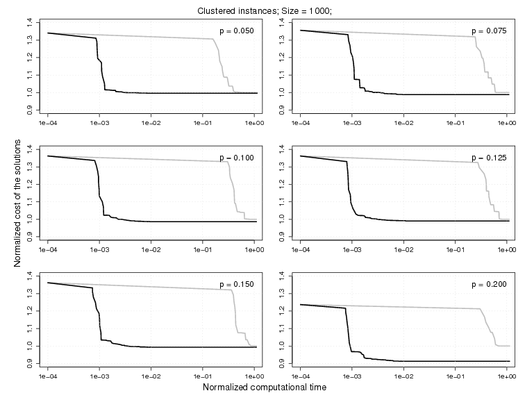
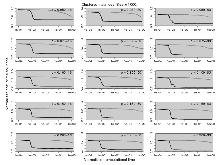
8. Experiments on iterated local search
Experimental results on
clustered homogeneous PTSP instances of size 1000 (300 KB). The plots represent the cost of the solutions obtained by ILS-2.5-opt-EEais normalized by the one obtained by ILS-2.5-opt-ACs. The normalization is done on an instance by instance basis for 10 instances; the normalized solution cost and the computation time are then aggregated. Note that the x-axis shows the computation time in logarithmic scale.
 |
 |
Experimental results on
clustered heterogeneous PTSP instances of size 1000 (1.5 MB). The plots represent the cost of the solutions obtained by ILS-2.5-opt-EEais normalized by the one obtained by ILS-2.5-opt-ACs. The normalization is done on an instance by instance basis for 10 instances; the normalized solution cost and the computation time are then aggregated. Note that the x-axis shows the computation time in logarithmic scale and ILS-2.5-opt-ACs uses a library for arbitrary precision arithmetics. To emphasize this fact the backgrounds of the plots are gray.
 |
|
9. Numerical values and statistical results:
We also provide the absolute values for all the results in the form of tables. In these tables, we present the final solution quality and the corresponding computational time for each probabiltiy range. Moreover, in order to test that the observed difference between the cost of the solutions reached by the considered algorithms are significant in a statistical sense, we use a t test and we present the p-values obtained from the t-test. The results are composed in a single pdf file: