by Giovanni Pini
April 2013
Return to the main page
Section 6.4 - Experimental setup
Section 6.4.2 - Trajectory of a marXbot (video)
As mentioned in Section 6.4.2 of the thesis, the marXbots systematically drift towards the left-hand side with respect to the direction of motion. The following video shows the typical trajectory followed by a marXbot when the wheel speeds are set to the same value.

|
The video shows the trajectory of a marXbot when both wheel speeds are set to 0.1 m/s. In the first part of the video the robots goes backwards, in the second part it goes forwards. |
|
TOP
Section 6.5 - Validation of the System
Section 6.5 - Real-robot experiments, results of individual runs
A summary of the results of each experimental run can be found
in this page.
TOP
Section 6.5 - Real-robot experiments, video recordings
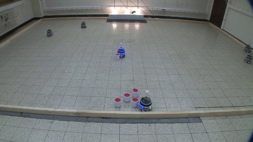
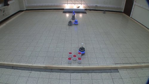
Video recordings of two experimental runs performed with the real marXbots are available:
|
The video shows a complete experimental run with the real marXbots. The robots perform foraging without using task partitioning. The experiment is divided into two phases of 15 minutes each. At the end of each phase, the robots' positions are marked on the arena floor, the batteries are changed, and the controller state is recorded so that it can be used to initialize the robots for the following phase. This is due to the high power consumption due to the extensive usage, made in the experiment, of the sensors and actuators available on the marXbot. This causes the battery to drain quickly with a consequent increase of hardware failures, which hinder the integrity of the experiments. Limiting the duration of each phase decreases considerably the frequency of failures due to low battery.
|
|
|
The video shows a complete experimental run with the real marXbots. The robots perform foraging using task partitioning. The experiment is divided into two phases of 15 minutes each. At the end of each phase, the robots' positions are marked on the arena floor, the batteries are changed, and the controller state is recorded so that it can be used to initialize the robots for the following phase. This is due to the high power consumption due to the extensive usage, made in the experiment, of the sensors and actuators available on the marXbot. This causes the battery to drain quickly with a consequent increase of hardware failures, which hinder the integrity of the experiments. Limiting the duration of each phase decreases considerably the frequency of failures due to low battery.
|
|
TOP
Section 6.5 - Simulation and real-robot experiments, comparison figures
The tables compare simulation and real-robot experiments. For each measure, we report the 95% confidence interval on the value of the mean. The first table reports the data collected in the experiments in which the swarm perform foraging using the non-partition strategy, while the second table reports the data collected in the experiments in which the swarm performs foraging using the partition strategy. The number of significant digits used to express frequencies depend on the total number of runs used to compute such frequencies (6 real-robot and 200 simulation runs for each strategy).
Non-partition strategy
| MEASURE | REAL ROBOTS | SIMULATION | DESCRIPTION |
| Get lost frequency - objects source | 0.7 - 0.8 | 0.77 - 0.79 | Frequency at which the robots do not locate the source during neighborhood search and gets lost |
| Source found with random walk | 0.7 - 0.8 | 0.77 - 0.79 | Frequency at which the source is found via random walk |
| Source found directly | 0.2 - 0.6 | 0.38 - 0.46 | Frequency at which the source is directly found: the duration of neighborhood search is zero |
| Exit arena | 0 - 0 | 0 - 0.02 | Number of times (per run) the robot tries to reach a position outside the boundaries |
Partition strategy
| MEASURE | REAL ROBOTS | SIMULATION | DESCRIPTION |
| Get lost frequency - objects source | 0.1 - 0.2 | 0.13 - 0.15 | Frequency at which the robots do not locate the source during neighborhood search and gets lost. |
| Source found with random walk | 0.1 - 0.2 | 0.21 - 0.23 | Frequency at which the source is found via random walk |
| Source found directly | 0.6 - 0.9 | 0.63 - 0.66 | Frequency at which the source is directly found: the duration of neighborhood search is zero |
| Get lost frequency - transfer locations | 0.1 - 0.2 | 0.11 - 0.12 | Frequency at which the robots do not locate the position where they received an object and get lost |
| Transfer partner found with random walk | 0.1 - 0.2 | 0.09 - 0.1 | Frequency at which a transfer partner is found via random walk |
| Transfer partner found directly - % | 0.3 - 0.4 | 0.14 - 0.16 | Frequency at which a transfer partner is directly found: the duration of neighborhood search is zero |
| Abandon transfer | 0.33 - 1.33 | 0.7 - 0.95 | Number of times (per run) the robots abandons trying to transfer the object (timeout) |
| Exit arena | 0 - 0.5 | 0 - 0 | Number of times (per run) the robot tries to reach a position outside the boundaries |
TOP
Section 6.6 - Simulation Experiments and Results
Section 6.6.1 - Effect of odometry error and swarm size
The following plot reports the performance of the fixed partitioning algorithms for different swarm sizes and values of the odometry error parameter.
Click
here to open.
TOP
Section 6.6.1 - Selection of the parameters epsilon and alpha
The following plots report the performance of the cost-based partitioning algorithm obtained with different settings of the parameters alpha and epsilon. Each plot reports the performance for a given value of epsilon and different values of alpha, number of robots and odometry error parameter.
Click on a link to open the corresponding plot:
Epsilon = 0.0Epsilon = 0.05Epsilon = 0.15Epsilon = 0.25Epsilon = 0.5
TOP