by Giovanni Pini
April 2013
Return to the main page
Section 5.2 - Experimental setup
Section 5.2 - Implementation of the cache using TAMs
|
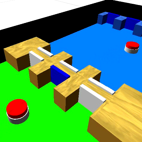
The video shows how the cache has been implemented using paired TAMs. Note that the video was produced using an older version of ARGoS, with respect to the one utilized to carry out the experiments presented in the thesis. However, the cache working principle remains the same.
|
|
Section 5.4 - The AdHoc Algorithm
Section 5.4.2 - Selection of the parameters of the AdHoc algorithm
To select the values of the parameters for the AdHoc algorithm, we perform experiments in which we change the value of the interfacing time during the course of the experimental run. Π is initialized to 160 seconds and it is set to 0 when the experimental run reaches its half. We test different combinations of the parameters with the goal of selecting a set of values that: i) allows the robots to properly select between the cache and the corridor and ii) renders the choice flexible and responsive to changes occurring in the environment. The following table reports the parameters and the values they assume in the different experiments.
| PARAMETER | TESTED VALUES |
| S | 0.5, 0.75, 1.0, 1.5, 2, 3 |
| α | 0.25, 0.5, 0.75 |
| O | -0.5, -1, -2, -3 |
| K | -0.5, -1, -2, -3 |
The following plots report the behavior of the AdHoc algorithm for different settings of the parameters. Each plot reports, for a given parameter setting, the percentage of usage of the cache and the corridor in time. Each plot reports the data collected in 25 experimental runs. Each box in the plot reports the percentage of usage of the cache during the 60 minutes preceding the time reported on the X axis. During the first half of experiment the performance is maximized if the robots do not utilize the cache. Conversely, in the second half of the experiment the maximal performance is reached if the all robots utilize the cache (ideally half of the swarm should work on each side).
Each figure reports, for a given setting of the parameters S and alpha, the results obtained for different values of the parameters O and K. Refer to Section 5.4.1 of the thesis for more details about the parameters of the AdHoc algorithm.
| | PARAMETER S |
| | 0.5 | 0.75 | 1.0 | 1.5 | 2 | 3 |
| ALPHA | 0.25 | α = 0.25, S=0.5 |
α = 0.25, S=0.75 |
α = 0.25, S=1.0 |
α = 0.25, S=1.5 |
α = 0.25, S=2.0 |
α = 0.25, S=3.0 |
| 0.5 | α = 0.5, S=0.5 |
α = 0.5, S=0.75 |
α = 0.5, S=1.0 |
α = 0.5, S=1.5 |
α = 0.5, S=2.0 |
α = 0.5, S=3.0 |
| 0.75 | α = 0.75, S=0.5 |
α = 0.75, S=0.75 |
α = 0.75, S=1.0 |
α = 0.75, S=1.5 |
α = 0.75, S=2.0 |
α = 0.75, S=3.0 |
We visually inspected the results reported in the figures, in order to select a set of values for the parameters. The results of the experiments suggest that S should be set to a high value. We select the value of 2, which corresponds to a higher degree of exploration with respect to the maximum tested value of 3. Concerning the value of alpha, the best results are obtained with a value of 0.5. Likely, the value 0.75 renders the algorithm sensitive to noise, while the value 0.25 impacts negatively the responsiveness of the algorithm. For both K and O, the results of the experiments suggest a value of -2 or -3. We selected for both -2, to avoid the extreme value -3 which seems in some cases to result in a poor flexibility with respect to changes of the value of Π.
TOP
Section 5.4.2 - Drop Abandon Statistics
We report here plots analogous to the ones reported in Figures 5.13 to 5.16 of the thesis. Each time a robot abandoned the choice of using the cache to drop an object, we recorded the number of empty cache TAMs (source side only) and the number of robots that were picking up objects (i.e., that were on the other side of the cache). The main plot in each figure is the histogram of the number of empty TAMs available at the cache when the robot abandoned (i.e., of positions where the robot could have dropped the object). The smaller plots at the bottom are histograms of the number of robots that were on the other side of the cache, picking up objects. Each of these histograms reports a subset of the data, corresponding to a given number of TAMs available at the cache. Thus, the first plot on the left indicates the number of robots that were picking up objects from the cache when a robot abandoned dropping and the no TAM was available at the cache. The second plot indicates analogous data, but for the cases in which there was one TAM available in the cache. The third plot for the cases in which there were two available TAMs. We collected the data in swarms of 4, 6, 8, and 10 robots using the AdHoc algorithm. Each figure can be opened by clicking on the corresponding link:
Swarm size: 4
Swarm size: 6
Swarm size: 8
Swarm size: 10
TOP
Section 5.5 - Task Partitioning as a Multi-armed Bandit Problem
Section 5.5.2 - Selection of the parameters
For each algorithm (AdHoc, UCB, and ε-Greedy) we test 10 different values for the corresponding parameter. Additionally, we test the two methods to compute the threshold used by the abandoning mechanism (refer to section 5.5.1 of the thesis). Therefore a total of 20 versions of each algorithm are tested.
In a first group of experiments, we fix the cache interfacing time to a certain value and we do not change this value during the experimental run. We test 7 values for the cache interfacing time: 0, 5, 10, 20, 40, 80, and 160 seconds. The following plots report the performance of the algorithms for the different values of the parameters and of the interfacing time. The performance is normalized. A value of 1 corresponds to the maximum performance that can be reached with the given interfacing time. This maximum has been determined empirically, by assigning robots a priori to each side of the cache and in the corridor and trying all the possible combinations. A value of performance of 0 corresponds to the performance obtained when the robots randomly select between the cache and the corridor with equal probability. Note that the normalized performance can be less than zero: this happens if the algorithm performs worse than the random choice.
Click on a link to open the corresponding plot:
AdHoc algorithm
ε-Greedy algorithm
UCB algorithm
In a second group of experiments, we change the value of Π during the course of the experimental run. We initialize Π to 160 seconds and set it to 0 seconds when the run reaches its half (after 5 hours). The following plots report the normalized performance (see description of above plots). The top plot in each figure reports the performance in the first half of the experiment, the bottom plot the performance in the second half.
Click on a link to open the corresponding plot:
AdHoc algorithm
ε-Greedy algorithm
UCB algorithm
TOP
Section 5.6 - The Use of Communication
Section 5.6.2 - Cache usage in time
The following plots report the usage of the cache in time, for the social versions of the studied algorithms. We report here the results of the experiments in which we initialize Π to 160 seconds and set it to 0 seconds when the experimental run reaches a quarter of its duration. In each plot, the vertical blue line marks the instant in which the value of Π changes. Archives containing the plots (1 file for each of the 100 experimental runs) can be accessed here:
AdHoc algorithm
ε-Greedy algorithm
UCB algorithm
TOP