Supplementary material for the paper:
Self-organized task allocation to sequentially interdependent tasks in swarm robotics
by Arne Brutschy, Giovanni Pini, Carlo Pinciroli, Mauro Birattari, and Marco Dorigo
Last change: September 24th, 2012
Abstract
In this article we present a self-organized method for allocating the individuals of a robot swarm to tasks that are sequentially interdependent. Tasks that are sequentially interdependent are common in natural and artificial systems. The proposed method does neither rely on global knowledge nor centralized components. Moreover, it does not require the robots to communicate. The method is based on the delay experienced by the robots working on one subtask when waiting for input from another subtask. We explore the capabilities of the method in different simulated environments. Additionally, we evaluate the method in a proof-of-concept experiment using real robots. We show that the method allows a swarm to reach a near-optimal allocation in the studied environments, can easily be transferred to a real-world setting, and is adaptive to changes in the properties of the tasks such as their duration. Finally, we show that the ideal setting of the parameters of the method does not depend on the properties of the environment.
Keywords: Swarm robotics, foraging, self-organization, task allocation, swarm intelligence, multi-agent systems.
Q-Q Plots of prey/ratio distribution
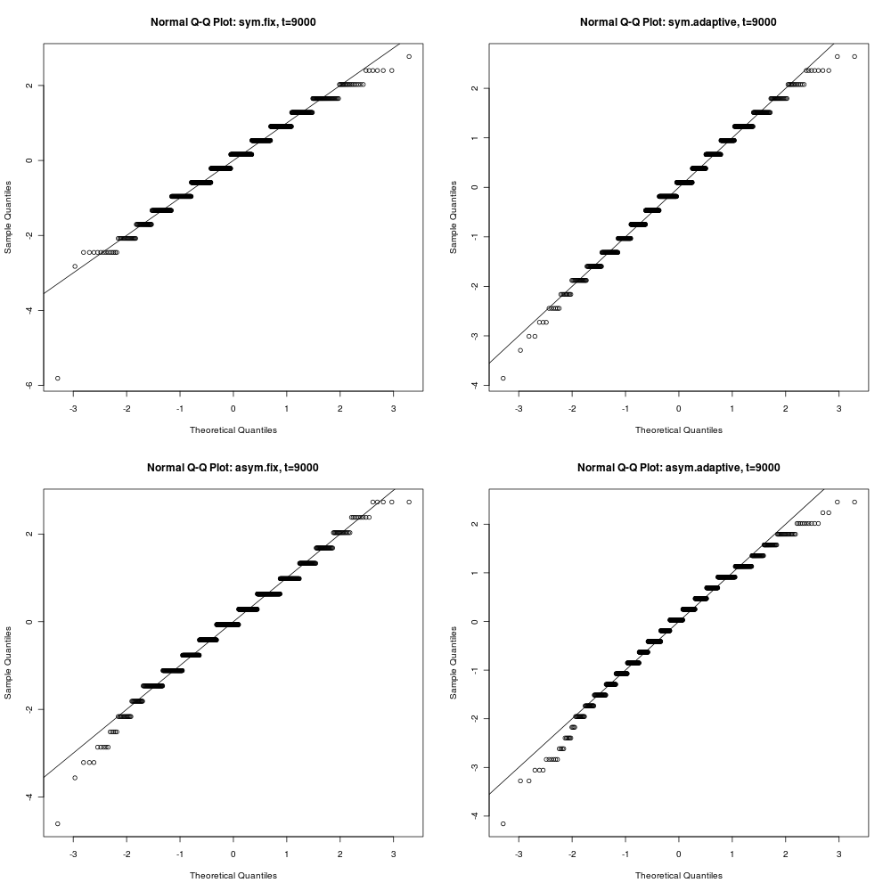 Figure s1a: Q-Q Plot for distribution of the group performance P as the number of prey objects collected at the middle of the experiment (t=9000). Fixed allocation
(left) and adaptive allocation (right) for the symmetric environment (top) and the asymmetric
environment (bottom). Apart from being a discrete random varible, P is not normally distributed, especicially in the case of the asymmetric environment.
Figure s1a: Q-Q Plot for distribution of the group performance P as the number of prey objects collected at the middle of the experiment (t=9000). Fixed allocation
(left) and adaptive allocation (right) for the symmetric environment (top) and the asymmetric
environment (bottom). Apart from being a discrete random varible, P is not normally distributed, especicially in the case of the asymmetric environment.
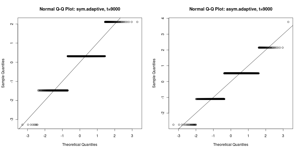 Figure s1b: Q-Q Plot for distribution of the allocation ratio R at the middle of the experiment (t=9000), for the symmetric
environment (left) and the asymmetric environment (right). Apart from being a discrete random varible,
R is not normally distributed, especicially in the case of the asymmetric environment.
Figure s1b: Q-Q Plot for distribution of the allocation ratio R at the middle of the experiment (t=9000), for the symmetric
environment (left) and the asymmetric environment (right). Apart from being a discrete random varible,
R is not normally distributed, especicially in the case of the asymmetric environment.
Comparison values for P
We measure the group performance P as the number of prey objects collected by the swarm at the end of the experiment. The group performance is used to evaluate the quality of the allocation of individuals to tasks: the higher the group performance, the better the quality of the allocation. We define three comparison values for the performance P:
- P_opt_N: maximum number of prey objects that can be harvested by a group of 18 robots when collisions are disabled (i.e., robots can move one through the other) and the task is not partitioned;
- P_nop_N: maximum number of prey objects that can be harvested by a group of 18 robots when collisions are enabled and the task is not partitioned;
- P_max_N: maximum number of prey objects that can be harvested by a group of N robots when collisions are enabled, the task is partitioned, and the robots are statically allocated (i.e., task switches are disabled) in an optimal way;
P_opt_18 is an unattainable value that gives an upper limit on the performance of a group of 18 robots, P_nop_18 allows to quantify the effect of interference between robots, and P_max_18 indicates the maximum value that can be achieved by a partitioned system.
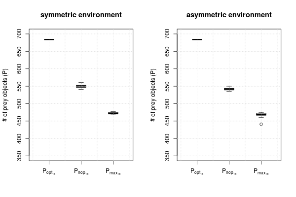 Figure s2: Comparison values for P when using 18 robots in the symmetric and asymmetric environments, obtained
empirically using a fixed optimal allocation.
Figure s2: Comparison values for P when using 18 robots in the symmetric and asymmetric environments, obtained
empirically using a fixed optimal allocation.
Task switching cost
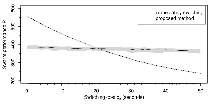 Figure s4 (analogously to Figure 7 in the paper): The effect of the switching cost c_s on the performance P of the system in the symmetric environment, evaluated using two different swarms: 1) in which robots always switch from subtask to subtask, and 2) in which robots use the proposed method to reach a stable allocation of robots to subtasks. Results are given as observation median (black line) and the 25%-75% quantiles (grey area).
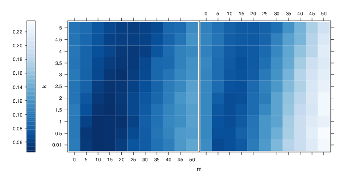
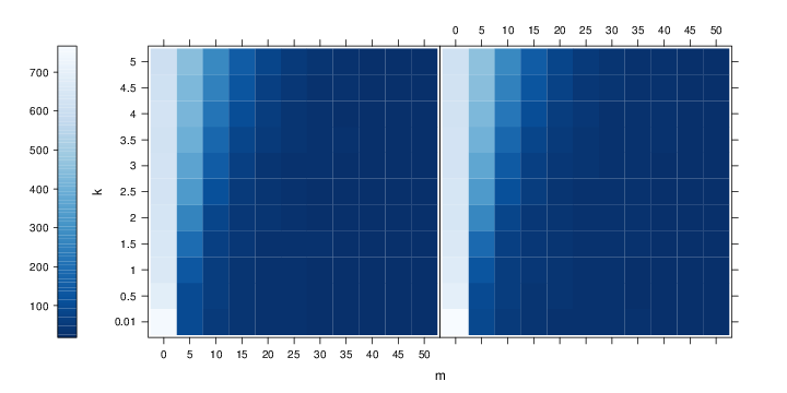
Effect of parameters k and m
Exhaustive search of the parameter space. The parameter k (steepness) is varied in the interval [0,5] by steps of 1, and the parameter m (shift) is varied in the interval [0,50] by steps of 5.
a)
 b)
b)
 c)
c)
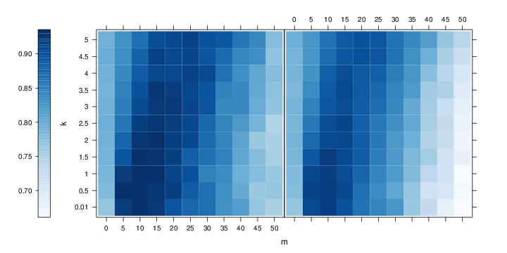 Figure s5a-c (Figure 8 in the paper, shown here because of colors): The effect of the parameters k (steepness) and m (shift)
as evaluated by the metrics a) mean absolute error, MAE, b) the total
number of switches between subtasks, S_total, and c) amount
of objects harvested, P, relative the the maximal performance P_real_18.
Left plots show the results for the symmetric environment, right plots
for the asymmetric environment. Darker squares indicate better values.
Figure s5a-c (Figure 8 in the paper, shown here because of colors): The effect of the parameters k (steepness) and m (shift)
as evaluated by the metrics a) mean absolute error, MAE, b) the total
number of switches between subtasks, S_total, and c) amount
of objects harvested, P, relative the the maximal performance P_real_18.
Left plots show the results for the symmetric environment, right plots
for the asymmetric environment. Darker squares indicate better values.
Influence of m in symmetric environment
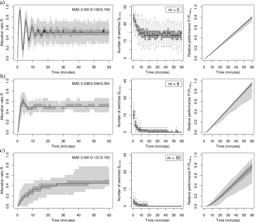 Figure s6 (analogously to Figure 9 in the paper):
Influence of the shift parameter m = {0, 8, 50} shown in a, b, and c, respectively. The experiment shown is conducted in the symmetric environment and evaluated using the three metrics. Left: allocation ratio R, given as observation median (black line) and the 1%-99% quantiles (grey area). The horizontal dotted line at R_opt = 0.5 indicates the optimal allocation for this environment. Middle: number of switches between subtasks for a time-window of 2min, S_2min. Right: amount P of objects harvested, relative the the maximal performance P_real_18, again as observation median and the 1%-99% quantiles.
Figure s6 (analogously to Figure 9 in the paper):
Influence of the shift parameter m = {0, 8, 50} shown in a, b, and c, respectively. The experiment shown is conducted in the symmetric environment and evaluated using the three metrics. Left: allocation ratio R, given as observation median (black line) and the 1%-99% quantiles (grey area). The horizontal dotted line at R_opt = 0.5 indicates the optimal allocation for this environment. Middle: number of switches between subtasks for a time-window of 2min, S_2min. Right: amount P of objects harvested, relative the the maximal performance P_real_18, again as observation median and the 1%-99% quantiles.
Scalability symmetric environment
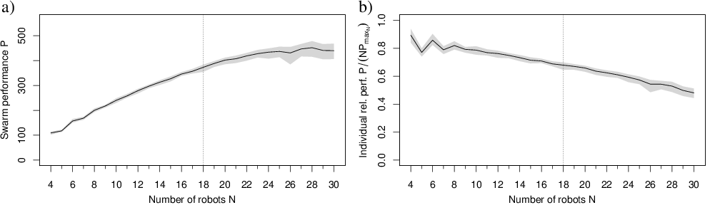 Figure s7 (analogously to Figure 10 in the paper): Scalability of the system for different group sizes for a swarm using the proposed method in the symmetric environment. a) Absolute performance P of the group as the number of objects harvested. b) Individual performance, P/P_real_N. As it can be seen, the performance of the group scales near-linearly. The absolute performance drops with increasing group size (most likely because of interference), while at the same time the spread of the distribution increases. Results are given as observation median (black line) and the 25%-75% quantiles (grey area). The vertical grey line at $N=18$ marks the group size used in all the other experiments.
Adaptivity asym. -> sym. environment
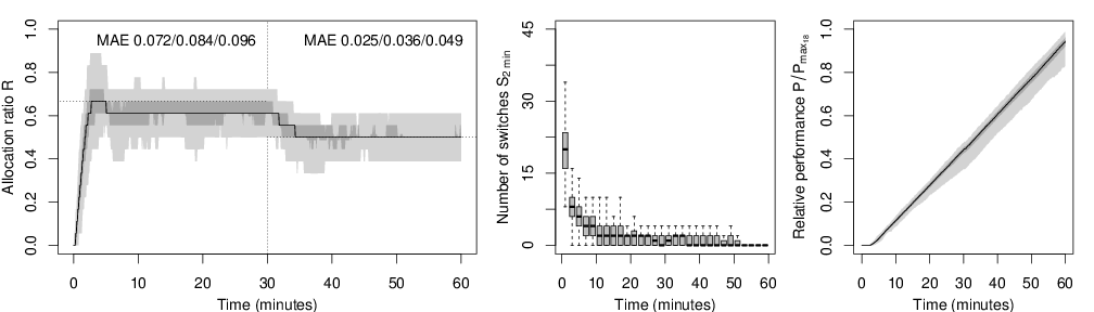 Figure s8 (analogously to Figure 11 in the paper): Adaptivity of the system when changing from the asymmetric environment to the symmetric environment at t = 30min. Left: allocation ratio R, given as observation median (black line) and the 1%-99% quantiles (grey area). The horizontal dotted line indicates the optimal allocation for each environment (at R_opt = 0.67 and 0.5, respectively) . Middle: number of switches between subtasks for a time-window of 2min, S_2min. Right: amount P of objects harvested, relative the the maximal performance P_real_18, again as observation median and the 1%-99% quantiles.
Real robot LED signals explained
In this Section, we explain the LED signals used between the robot and an active prey object.
We use the object in an active way: objects and robots exchange information with each other, by means of active LED signaling. The use of active signaling simplified the implementation of the controller in an aspect that is not relevant for the task allocation problem. Signaling is used only between an object and a robot, and never between two robots. While the robot is fully autonomous in its behavior, the object signals are activated by a human-controlled program that triggers the transitions between the different states.
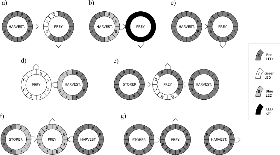
Figure s9: Representation of the visual signals exchanged between prey objects and robots, from the moment a prey object is harvested in the source till the moment it leaves the exchange zone after a successful transfer. The LED ring of the robot is divided in 8 sectors, each corresponding to one of the LEDs. Dark grey, light grey and white sectors represent red, blue, and green LEDs, respectively. Black sectors represent LEDs turned off. The robot's forward direction is shown by a stylized representation of the gripper. Please refer to the text below for what concerns the meaning of each signal.
Figure s9 shows the sequence of events happening from the moment a prey object is harvested from the source by a harvester, till the moment the same prey object is handed over to a storer in the exchange zone. In general, a green LEDs stands for the willingness to connect, while red is used as repel colour that other robots try to avoid.
- At the beginning, the prey object is in the source, with 3 LEDs lit up in green, and the rest in red. The harvester, fully lit in red, is approaching the prey object.
- When the harvester managed to grip the prey object, it turns its front LEDs to blue to signal it is ready to leave the source. The prey object then turns off the LEDs and only then the harvester starts moving towards the exchange zone.
- While pulling the object to the exchange zone, the harvester and the prey object are fully lit up in red to signal their presence to other robots.
- Once it reaches its destination, the prey object has to be turned by 180 degrees in order to make it easier for a storer to approach and grip it. When the turning of the prey object is done, the harvester lights up the 4 front LEDs in blue, and the prey object answers by lighting up in green.
- When the harvester perceives that the prey object has turned green, it is ready for handing the prey object over to a storer. The harvester turns the LEDs to red and the prey object lights half of the ring in red, and the other half in green to invite storers to connect.
- When a storer connects to the prey object, it signal this event by turning the 4 front LEDs to blue, and the prey turns in blue to signal the storer and the harvester that the transfer was completed.
- The harvester then goes back to the source to search for more prey objects, and the storer to the nest, to store the prey object it just received.
Real robot video
This video shows the recorded real robot experiment: (left) a harvester is retrieving a prey object from the source; (middle) a storer and a harvester are transferring a prey object in the exchange zone; (right) a storer is dragging a prey object into the nest. Prey objects are marked by a grey circle on top.
The goal of this experiment is to validate the method proposed in this work in a real world setting. The results presented in this section serve as \proof-of-concept", showing that the method for task allocation can be transferred with success to real robots.
At the beginning of the experiment, 4 s-bots are randomly positioned in the harvest area and 4 prey objects are positioned in the source, close to the border of the environment. At the end of each segment, the experiment is stopped, the controller state is saved and the robots batteries are recharged. We divided the experiment in 18 segments of 5 minutes each, for a total run time of 90 minutes. At the beginning of each segment the robots are placed at the same position they had at the end of the previous segment, and the internal state of the controllers is restored. The controllers use the parameter values determined in the simulation experiments, m = 8 and k = 1.
During the course of the 90 minutes experimental run, the robots harvested 40 prey objects.
Download the video:
Statistical analysis results
Download all results of the statistical analysis (obtained using R):