by Giovanni Pini, Arne Brutschy, Gianpiero Francesca, Marco Dorigo, and Mauro Birattari
DATE: March 2012
|
Table of Contents |
VIDEO - IMPLEMENTATION OF THE CACHE USING THE TAM
|
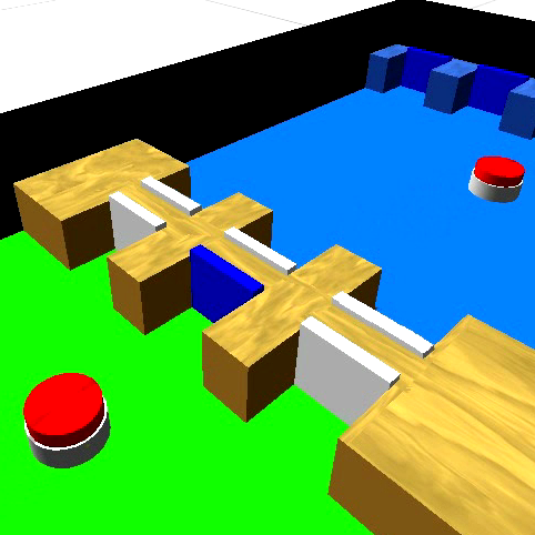
The video explains how object transfer through the cache is implemented using the TAM. For more information about the TAM, please refer to the technical report 2010-015, and to the information that can be found here. In the video, e-pucks carrying objects are colored in red. Please notice that the video was created with a previous version of ARGoS. |
TOP
WAYS OF COMPUTING THE THRESHOLD FOR THE GIVEUP MECHANISM
Here we describe how the give up threshold is computed. This threshold is used in the give up mechanism, decribed at the end of Section 3 of the paper.Give up threshold T1
In this case, the there is a threshold used when picking up objects from the cache, and another one when dropping. When dropping objects in the cache, the threshold is computed as three times the estimate of the cost needed to drop objects, computed using Equation 1 of the paper. Analogously for picking up objects from the cache the threshold is three times the estimate cost of picking up objects from the cache.Give up threshold T2
In this case, the there is only one threshold that is used on both sides of the cache. The threshold is computed as three times the average of the estimates of the cost needed to pick up and drop objects, computed using Equation 1 of the paper.Give up threshold T3
In this case, the there is only one threshold that is used on both sides of the cache. The threshold is computed according to Equation 1 of the paper, but without making a distinction between pick up and drop times: both pick up and drop times measures are used to compute a single value. That value, multiplied by 3, is then the value of the threshold for the give up mechanism.TOP
FIRST SET OF EXPERIMENTS - SUPPLEMENTARY PLOTS
The goal of the first set of experiments is to select the parameter values to be used with each algorithm. We test the algorithms in the normal corridor and long corridor environments, with swarms composed of 10 and 20 robots.For each algorithm, we test 10 possible values of the corresponding parameter:
| ALGORITHM | PARAMETER VALUES |
| Ad-Hoc | Parameter S = {0.5, 0.75, 1.0, 1.25, 1.5, 2.0, 3.0, 4.0, 5.0, 6.0} |
| UCB | Gamma = {100, 250, 500, 1000, 2000, 4000, 6000, 8000, 10000, 15000} |
| ε-greedy | ε = {0.01, 0.02, 0.05, 0.08, 0.11, 0.14, 0.17, 0.20, 0.25, 0.28} |
Additionally, we test for each the three possible ways of computing the giveup threshold (as described here).
We perform two types of experiments. In the experiments of the first type, the cache interfacing time Π is fixed to a value and does not change during the experiments. We selected 7 different values for the cache interfacing time: 0, 5, 10, 20, 40, 80, and 160 seconds.
In the the second type of experiments, the cache interfacing time Π is initialized to 160 seconds and changes when the experiment reaches its half (after 5 hours).
Experiment type 1: constant value of cache interfacing time Π
In each file, the left column reports the plots for the swarm composed of 10 robots, the right column for the one composed of 20 robots. Each row corresponds to a value of the cache interfacing time Π. Different colors of the boxes represent the 3 different ways for computing the giveup threshold. For each color there are 10 bars, one for each value of the algorithm's parameter.The plots report the performance of the algorithms, for each value of the algorithm's parameter. The performance is normalized. A value of 1 corresponds to the maximum performance that can be achieved in the corresponding setting (environment, number of robots, interfacing time). The maximum has been determined empirically, by manually assigning robots to each side of the cache or the corridor and trying all the possible combinations. A value of 0 in performance corresponds to the performance of a naive algorithm in which the robots randomly select between the cache and a corridor, without using the information about the cost estimates. An algorithm's performance can be less than zero if it performs worse than the naive algorithm.
A plot can be opened in a fresh tab by clicking on the correcponding link:
ad-hoc algorithm, long corridor environment
ad-hoc algorithm, short corridor environment.
UCB algorithm, long corridor environment
UCB algorithm, short corridor environment.
ε-greedy algorithm, long corridor environment
ε-greedy algorithm, short corridor environment.
Experiment type 2: variable value of cache interfacing time Π
In each file, the results of the experiment with varying Π The plots in the left column report the reults for the swarm of 10 robots, the one on the right for the swarm composed of 20 robots. The first row reports the normalized performance (see above for the case with constant interfacing time Π) during the first half of experiment, the second row the one during the second half (after the change in Π occurred). Different colors of the boxes represent the 3 different ways for computing the giveup threshold. For each color there are 10 bars, one for each value of the algorithm's parameter.A plot can be opened in a fresh tab by clicking on the correcponding link.
ad-hoc algorithm, long corridor environment
ad-hoc algorithm, short corridor environment.
UCB algorithm, long corridor environment
UCB algorithm, short corridor environment.
ε-greedy algorithm, long corridor environment
ε-greedy algorithm, short corridor environment.
TOP
Selected values of the parameters
The results of experiments of type 1 suggest values of the parameters that render the corresponding algorithm exploiting. Therefore the parameter S should be 6 for the ad-hoc algorithm, gamma should be 100 for UCB, and ε 0.01 for the ε-greedy. This is due to the fact that the value of Π is constant in time, therefore no exploration is needed. Once the robot determined whether it is better to employ task partitioning or not, they should never change decision.The results of experiments of type 2 suggest intermediate values for each algorithm. A good balance between exploration and exploitation must be found. Too much exploration does not allow to exploit task partitioning effectively. Too much exploitation does not allow to detect changes occurring in the environment, and also lead to poor performance.
The effect of way of computing the give up threshold is different from algorithm to algorithm. The fllowing table summarizes the algorithms' parameters employed in the paper:
| ALGORITHM | PARAMETER VALUE | THRESHOLD COMPUTING |
| Ad-Hoc, exploiting version | Parameter S = 6.0 | Give up threshold T3 |
| Ad-Hoc, exploring version | Parameter S = 1.0 | Give up threshold T3 |
| UCB, exploiting version | Gamma = 100 | Give up threshold T3 |
| UCB, exploring version | Gamma = 1000 | Give up threshold T1 |
| ε-greedy, exploiting version | ε = 0.01 | Give up threshold T1 |
| ε-greedy, exploring version | ε = 0.11 | Give up threshold T1 |
TOP
SECOND SET OF EXPERIMENTS - SUPPLEMENTARY PLOTS
The goal of the second set of experiment is to assess whether the algorithms are able to choose properly between partitioning the task or not, on the basis of the value of Π. The algorithm should also be able to adapt to changes of Π. The value of Π switches between 0 and 160 (seconds). The initial value is 0; after 2.5 hours (1/4 of experiment), Π changes to 160 seconds and then it is seto back to 0 at half the experiment. Each file contains the results for the 2 versions of an algorithm, in a certain environment for the 2 swarm sizes. Each box of the plot reports the percentage of usage of the cache in the 30 minutes preceding the value reported on the X axis. The plot also reports the target optimal cache usage (red horizontal line), and an area in which the percentage is at least 95% of the maximum (red oblique lines). In some plots the red oblique lines are missing: in these cases, every cache usage that is not the optimal leads to a performance that is less than 95% of the maximum.A plot can be opened in a fresh tab by clicking on the correcponding link.
ad-hoc algorithm, long corridor environment
ad-hoc algorithm, short corridor environment.
UCB algorithm, long corridor environment
UCB algorithm, short corridor environment.
ε-greedy algorithm, long corridor environment
ε-greedy algorithm, short corridor environment.
TOP