
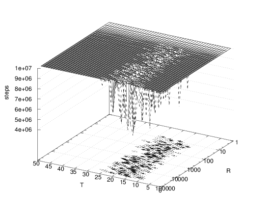
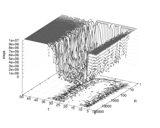
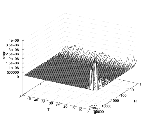
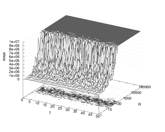
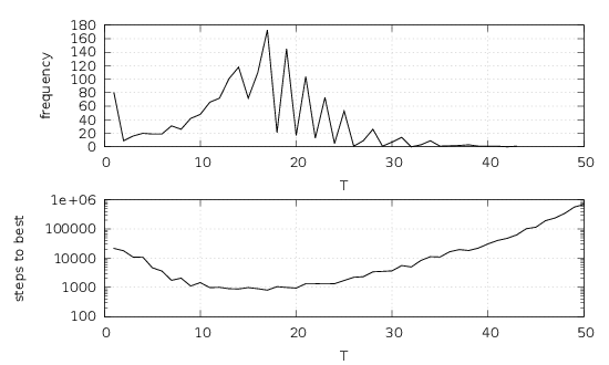
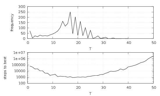
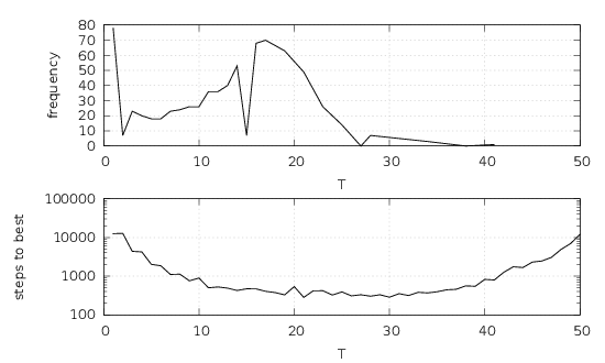
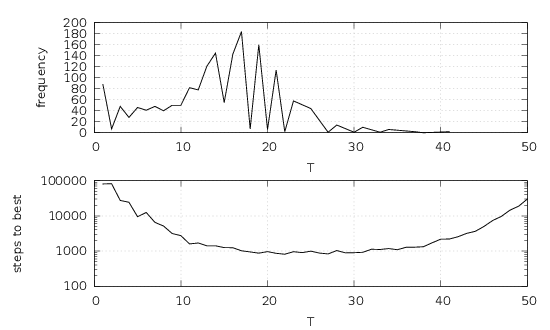
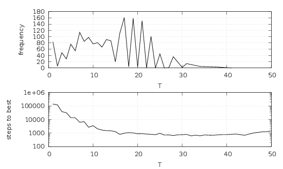
Figure 1: Median number of steps to find the optimal solution across 10 runs
of FixedTL-MCP, which corresponds to RTS-MCP with fixed parameter settings
on instance C500.9.


| Instance | RTS-MCP | Random[1,MAXT]-MCP
|
| C125.9 | 84.0 | 68.0 |
| C250.9 | 1 147.0 | 1 157.0 |
| C500.9 | 81 144.0 | 25 225.0 |
| C1000.9 | 708 530.0 | 348 284.5 |
| C2000.9 | 0.4% | 0.5% |
| DSJC1000.5 | 34 560.0 | 22 452.0 |
| DSJC500.5 | 1 400.5 | 1 347.0 |
| C2000.5 | 32 772.0 | 22 939.0 |
| C4000.5 | 3 677 632.0 | 2 356 013.0 |
| MANN_a27 | 75 262.0 | 62 760.0 |
| MANN_a45 | 0.2% | 0.2% |
| MANN_a81 | 0.2% | 0.1% |
| brock200_2 | 56 583.0 | 1 339 147.5 |
| brock200_4 | 178 136.0 | 2 067 906.0 |
| brock400_2 | 93.4% | 16.8% |
| brock400_4 | 100.0% | 99.4% |
| brock800_2 | 1.0% | 0.0% |
| brock800_4 | 14.5% | 2.2% |
| gen200_p0.9_44 | 1 429.0 | 1 825.0 |
| gen200_p0.9_55 | 584.0 | 709.0 |
| gen400_p0.9_55 | 21 150.5 | 27 503.0 |
| gen400_p0.9_65 | 1 390.0 | 1 374.0 |
| gen400_p0.9_75 | 1 583.0 | 1 417.0 |
| hamming10-4 | 491.0 | 530.0 |
| keller5 | 3 040.0 | 10 063.0 |
| keller6 | 672 768.0 | 1 010 057.0 |
| p_hat300-1 | 139.0 | 122.0 |
| p_hat300-2 | 27.0 | 29.0 |
| p_hat300-3 | 620.0 | 632.0 |
| p_hat700-1 | 1 182.0 | 1 473.5 |
| p_hat700-2 | 118.0 | 92.0 |
| p_hat700-3 | 210.0 | 204.0 |
| p_hat1500-1 | 139 617.0 | 153 983.0 |
| p_hat1500-2 | 363.0 | 254.0 |
| p_hat1500-3 | 1 229.0 | 708.0 |
| Instance | RTS-MCP | FixedTL-MCP
|
| C125.9 | 0.0 | 0.0 |
| C250.9 | 0.0 | 0.0 |
| C500.9 | 0.1 | 0.0 |
| C1000.9 | 1.1 | 0.5 |
| C2000.9 | 0.4% | 0.2% |
| DSJC1000.5 | 0.2 | 0.1 |
| DSJC500.5 | 0.0 | 0.0 |
| C2000.5 | 0.3 | 0.2 |
| C4000.5 | 50.8 | 53.9 |
| MANN_a27 | 0.1 | 0.1 |
| MANN_a45 | 0.2% | 0.1% |
| MANN_a81 | 0.2% | 0.0% |
| brock200_2 | 0.1 | 0.1 |
| brock200_4 | 0.2 | 0.1 |
| brock400_2 | 93.4% | 99.1% |
| brock400_4 | 1.3 | 1.1 |
| brock800_2 | 1.0% | 2.1% |
| brock800_4 | 14.5% | 21.6% |
| gen200_p0.9_44 | 0.0 | 0.0 |
| gen200_p0.9_55 | 0.0 | 0.0 |
| gen400_p0.9_55 | 0.0 | 0.0 |
| gen400_p0.9_65 | 0.0 | 0.0 |
| gen400_p0.9_75 | 0.0 | 0.0 |
| hamming10-4 | 0.0 | 0.0 |
| keller5 | 0.0 | 0.0 |
| keller6 | 4.9 | 3.9 |
| p_hat300-1 | 0.0 | 0.0 |
| p_hat300-2 | 0.0 | 0.0 |
| p_hat300-3 | 0.0 | 0.0 |
| p_hat700-1 | 0.0 | 0.0 |
| p_hat700-2 | 0.0 | 0.0 |
| p_hat700-3 | 0.0 | 0.0 |
| p_hat1500-1 | 1.3 | 1.0 |
| p_hat1500-2 | 0.0 | 0.0 |
| p_hat1500-3 | 0.0 | 0.0 |
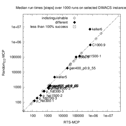
| Instance | RTS-MCP | RandomED-MCP
|
| C125.9 | 0.0 | 0.0 |
| C250.9 | 0.0 | 0.0 |
| C500.9 | 0.1 | 0.1 |
| C1000.9 | 1.1 | 0.9 |
| C2000.9 | 0.4% | 0.0% |
| DSJC1000.5 | 0.2 | 0.2 |
| DSJC500.5 | 0.0 | 0.0 |
| C2000.5 | 0.3 | 0.3 |
| C4000.5 | 50.8 | 78.5 |
| MANN_a27 | 0.1 | 0.1 |
| MANN_a45 | 0.2% | 0.1% |
| MANN_a81 | 0.2% | 0.0% |
| brock200_2 | 0.1 | 0.1 |
| brock200_4 | 0.2 | 0.2 |
| brock400_2 | 93.4% | 92.7% |
| brock400_4 | 1.3 | 2.0 |
| brock800_2 | 1.0% | 1.3% |
| brock800_4 | 14.5% | 14.0% |
| gen200_p0.9_44 | 0.0 | 0.0 |
| gen200_p0.9_55 | 0.0 | 0.0 |
| gen400_p0.9_55 | 0.0 | 0.0 |
| gen400_p0.9_65 | 0.0 | 0.0 |
| gen400_p0.9_75 | 0.0 | 0.0 |
| hamming10-4 | 0.0 | 0.0 |
| keller5 | 0.0 | 0.0 |
| keller6 | 4.9 | 50.6 |
| p_hat300-1 | 0.0 | 0.0 |
| p_hat300-2 | 0.0 | 0.0 |
| p_hat300-3 | 0.0 | 0.0 |
| p_hat700-1 | 0.0 | 0.0 |
| p_hat700-2 | 0.0 | 0.0 |
| p_hat700-3 | 0.0 | 0.0 |
| p_hat1500-1 | 1.3 | 1.0 |
| p_hat1500-2 | 0.0 | 0.0 |
| p_hat1500-3 | 0.0 | 0.0 |
| Instance | RTS-MCP | Random[1,MAXT]-MCP
|
| C125.9 | 0.0 | 0.0 |
| C250.9 | 0.0 | 0.0 |
| C500.9 | 0.1 | 0.0 |
| C1000.9 | 1.1 | 0.5 |
| C2000.9 | 0.4% | 0.5% |
| DSJC1000.5 | 0.2 | 0.1 |
| DSJC500.5 | 0.0 | 0.0 |
| C2000.5 | 0.3 | 0.2 |
| C4000.5 | 50.8 | 50.3 |
| MANN_a27 | 0.1 | 0.1 |
| MANN_a45 | 0.2% | 0.2% |
| MANN_a81 | 0.2% | 0.1% |
| brock200_2 | 0.1 | 1.5 |
| brock200_4 | 0.2 | 1.8 |
| brock400_2 | 93.4% | 16.8% |
| brock400_4 | 100.0% | 99.4% |
| brock800_2 | 1.0% | 0.0% |
| brock800_4 | 14.5% | 2.2% |
| gen200_p0.9_44 | 0.0 | 0.0 |
| gen200_p0.9_55 | 0.0 | 0.0 |
| gen400_p0.9_55 | 0.0 | 0.0 |
| gen400_p0.9_65 | 0.0 | 0.0 |
| gen400_p0.9_75 | 0.0 | 0.0 |
| hamming10-4 | 0.0 | 0.0 |
| keller5 | 0.0 | 0.0 |
| keller6 | 4.9 | 7.1 |
| p_hat300-1 | 0.0 | 0.0 |
| p_hat300-2 | 0.0 | 0.0 |
| p_hat300-3 | 0.0 | 0.0 |
| p_hat700-1 | 0.0 | 0.0 |
| p_hat700-2 | 0.0 | 0.0 |
| p_hat700-3 | 0.0 | 0.0 |
| p_hat1500-1 | 1.3 | 1.3 |
| p_hat1500-2 | 0.0 | 0.0 |
| p_hat1500-3 | 0.0 | 0.0 |
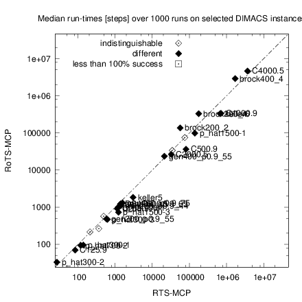
| Instance | RTS-MCP | RoTS-MCP |
| C125.9 | 0.0 | 0.0 |
| C250.9 | 0.0 | 0.0 |
| C500.9 | 0.1 | 0.0 |
| C1000.9 | 1.1 | 0.5 |
| C2000.9 | 0.4% | 0.9% |
| DSJC1000.5 | 0.2 | 0.2 |
| DSJC500.5 | 0.0 | 0.0 |
| C2000.5 | 0.3 | 0.3 |
| C4000.5 | 50.8 | 100.4 |
| MANN_a27 | 0.1 | 0.1 |
| MANN_a45 | 0.2% | 0.3% |
| MANN_a81 | 0.2% | 0.0% |
| brock200_2 | 0.1 | 0.2 |
| brock200_4 | 0.2 | 0.3 |
| brock400_2 | 93.4% | 76.4% |
| brock400_4 | 1.3 | 3.8 |
| brock800_2 | 1.0% | 0.5% |
| brock800_4 | 14.5% | 11.5% |
| gen200_p0.9_44 | 0.0 | 0.0 |
| gen200_p0.9_55 | 0.0 | 0.0 |
| gen400_p0.9_55 | 0.0 | 0.0 |
| gen400_p0.9_65 | 0.0 | 0.0 |
| gen400_p0.9_75 | 0.0 | 0.0 |
| hamming10-4 | 0.0 | 0.0 |
| keller5 | 0.0 | 0.0 |
| keller6 | 4.9 | 2.4 |
| p_hat300-1 | 0.0 | 0.0 |
| p_hat300-2 | 0.0 | 0.0 |
| p_hat300-3 | 0.0 | 0.0 |
| p_hat700-1 | 0.0 | 0.0 |
| p_hat700-2 | 0.0 | 0.0 |
| p_hat700-3 | 0.0 | 0.0 |
| p_hat1500-1 | 1.3 | 0.9 |
| p_hat1500-2 | 0.0 | 0.0 |
| p_hat1500-3 | 0.0 | 0.0 |