This page contains supplementary material for the paper "Task partitioning in swarms of robots: An adaptive method for strategy selection".
CONTENTS:
VIDEOS
This section contains videos that illustrate some specific aspects of the simulations.
|
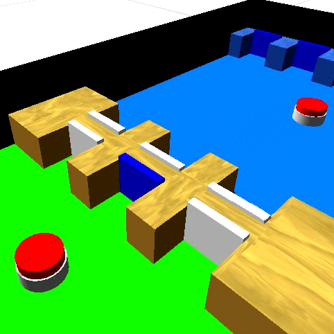
This video explains how object transfer through the cache is implemented using the booths. |
|
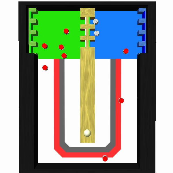
This videos shows how the experiment develops in time. Robots are red when carrying an object, gray when not. The graph on the right-hand side shows how the robot's choices evolve in time. The red curve is the percentage of selection of the cache in the previous 8 minutes, the blue curve the percentage of selection of the corridor. |
PLOTS
The plots here presented report all the data of the simulations, gathered using the following criteria:- Each experimental condition has been repeated 50 times, with a different seed for the random numbers generator.
- In the unlikely event in which a robot unintentionally entered a booth at the cache, the corresponding simulation data is discarded (as the cache would become inconsistent).
- A data point was collected every 20 simulated seconds.
The plots here presented are of four typologies:
- Paper plots: plots also found in the paper, but with 95% confidence intervals also plotted
- Throughput: report the throughput of the swarm in the course of the experiment.
- Strategy selection: report the strategy being selected by the swarm in time when the adaptive method is being used.
- Average times: report the average corridor and cache usage times using the different methods.
Paper plots
The following graph reports the performance of the three methods (adaptive, always-partition, and never-partition) for the different values of the interfacing time Π. The dashed lines around the main plot report 95% confidence intervals. Click on the plot to enlarge it.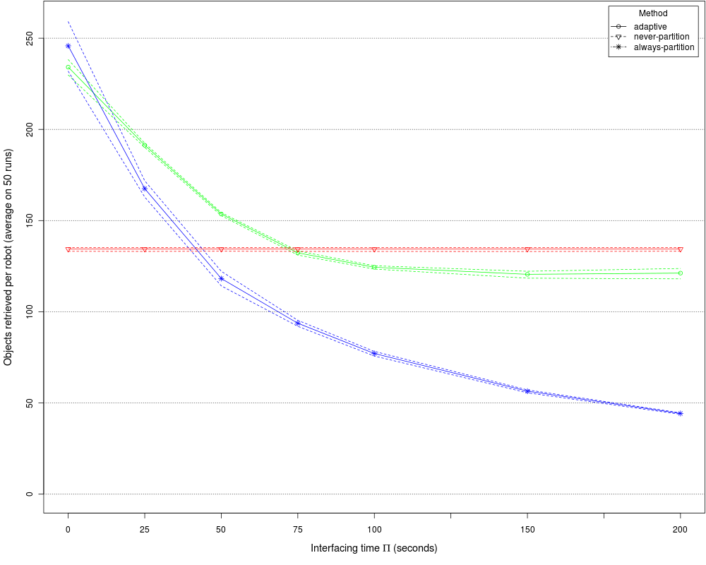 |
 |
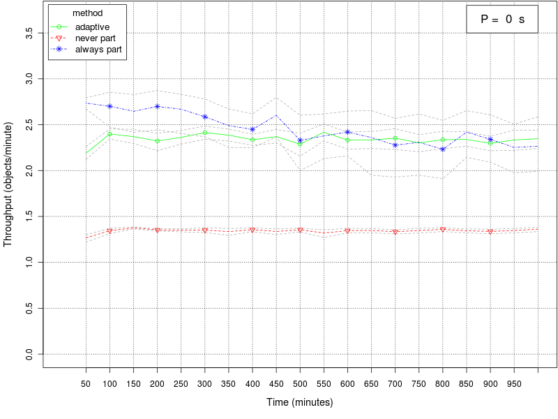
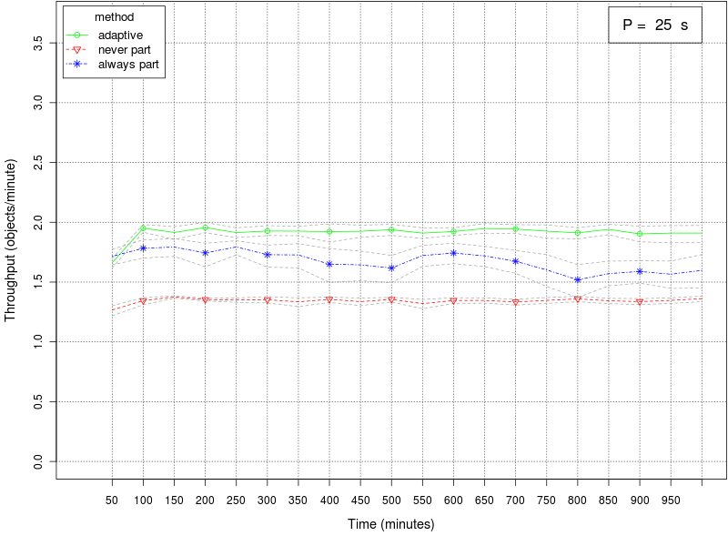
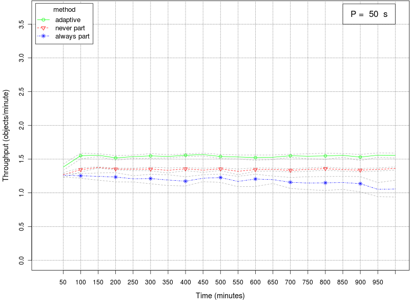
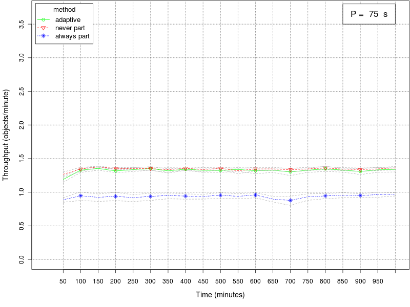
Throughput plots
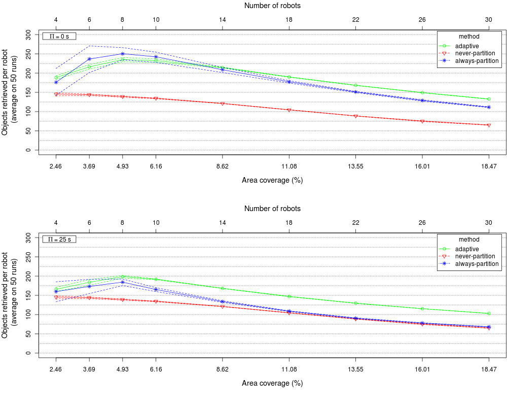
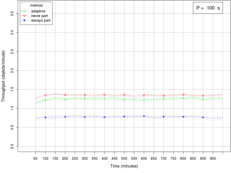
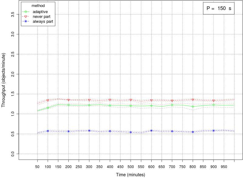
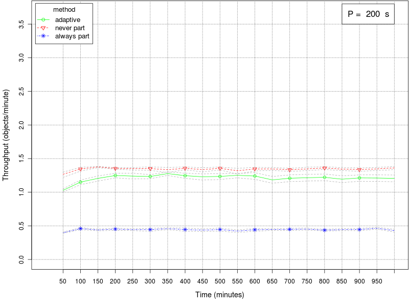
The following set of graphs plots the throughput of the swarm for different values of the interfacing time Π using the 3 different methods (always partition, never partition, and adaptive method). The interfacing time Π assumes the following values: 0, 25, 50, 75, 100, 150, and 200. The throughput is expressed as object retrieved per minute of simulated time. Each point in the graph plots the average throughput in the 15 minutes time window preceding the value reported on the X axis. The dashed gray lines around the main plot represent the 95% confidence interval on the observed mean.Click on a plot to enlarge it.
 |
 |
 |
 |
 |
 |
 |
| Plots index | Top |
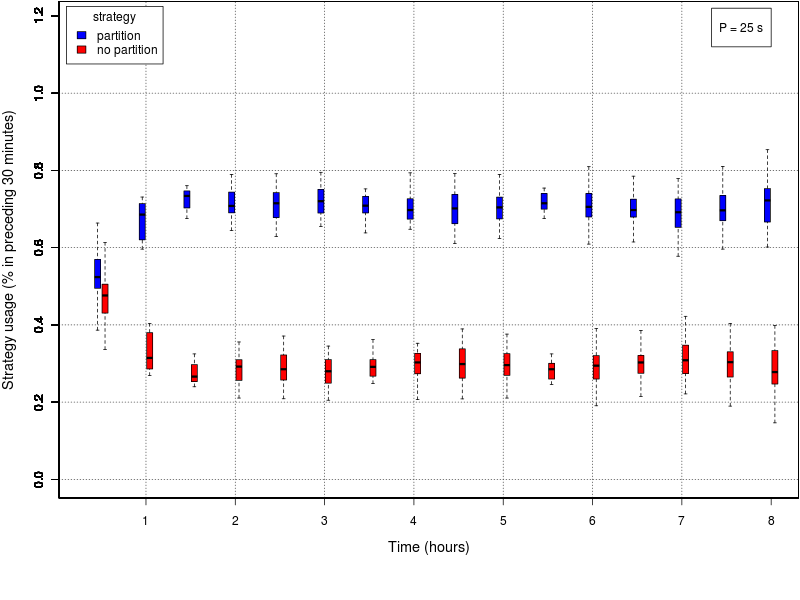
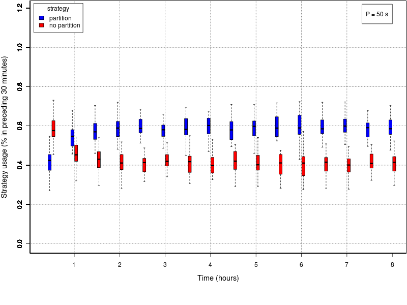
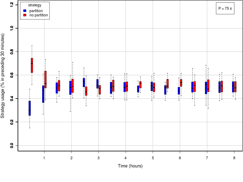
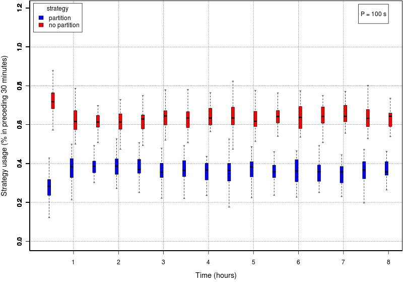
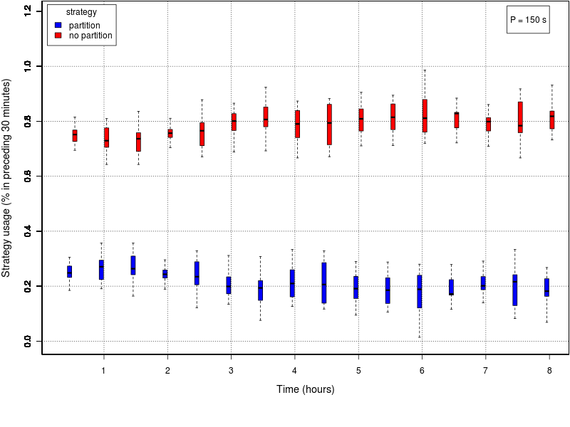
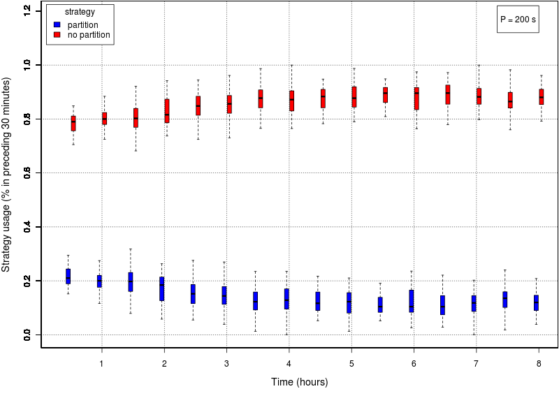
Strategy usage plots
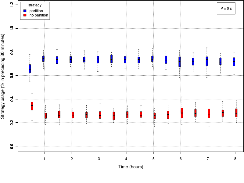
The following set of graphs plots the strategy used by the swarm in time for different values of the interfacing time Π using the adaptive method. The interfacing time assumes the following values: 0, 25, 50, 75, 100, 150, and 200. The data reported in all the plots is the one of the first half of the experiment (roughly 8 hours), as in all cases the method converged before half the experiment. The time period is divided into windows of 30 minutes; each box reports the percentage of usage of each strategy in the time window preceding the value reported on the X axis. The usage of the cooridor takes into account also the cases in which the robots initially selected the cache, but then gave up its usage.Click on a plot to enlarge it.
 |
 |
|
 |
 |
|
 |
 |
|
 |
| Plots index | Top |
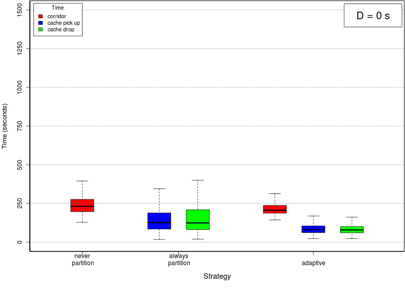
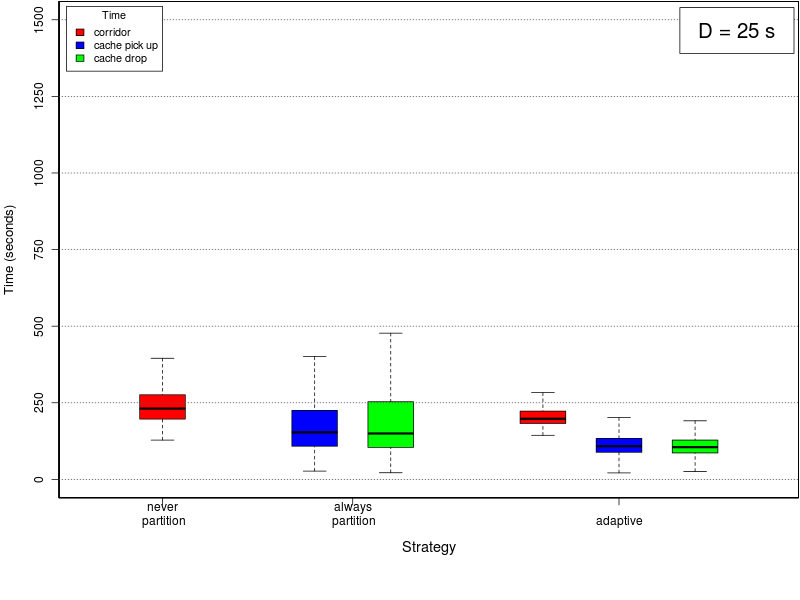
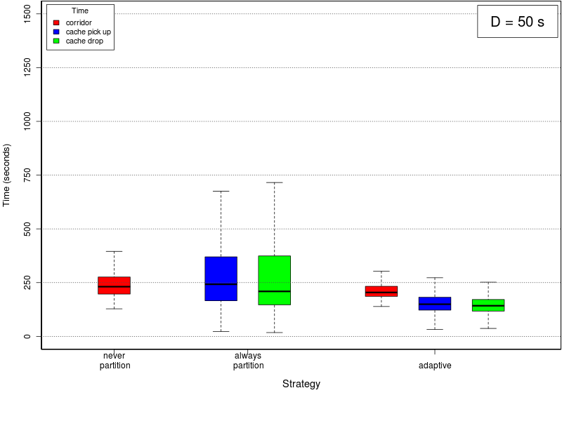
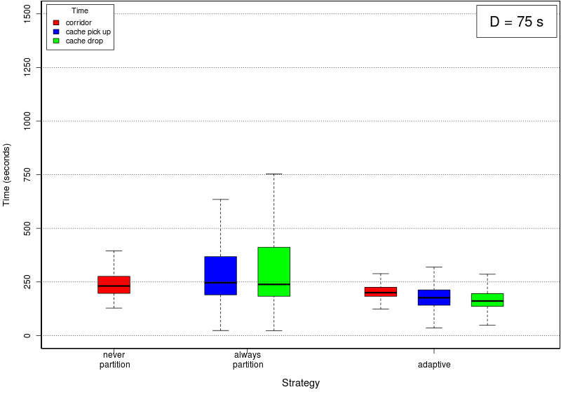
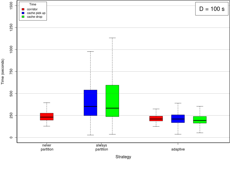
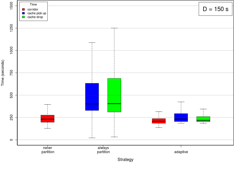
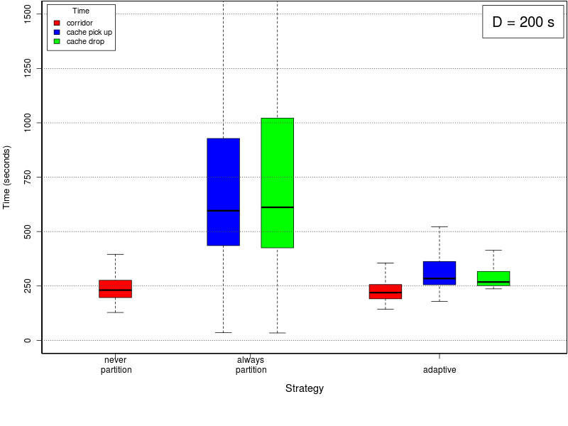
Average times plots
The following set of graphs plots the average time needed to use the corridor and the cache (for picking up and dropping objects) for different values of the interfacing time and for the threee methods. The interfacing time assumes the following values: 0, 25, 50, 75, 100, 150, and 200.Click on a plot to enlarge it.
 |
 |
 |
 |
 |
 |
 |
| Plots index | Top |
ANOVA
To study the effect of the parameters on the method proposed, we use a full factorial design. The chosen factor levels are the following:- Interfacing time Π: 0, 100, 200
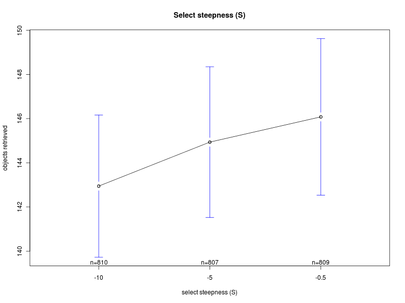
- Strategy selection steepness S: -0.5, -5, -10
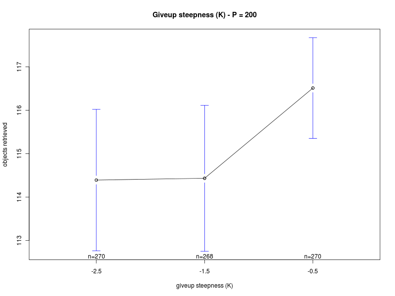
- Give up partitioning steepness K: -0.5, -1.5, -2.5
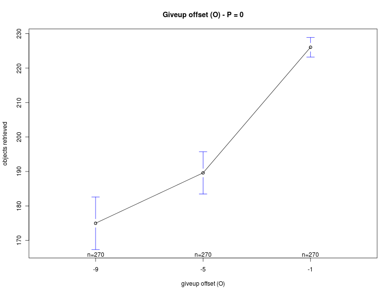
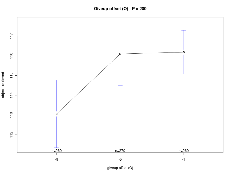
- Give up partitioning offset O: -1, -5, -9
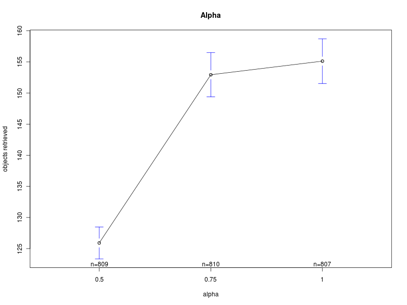
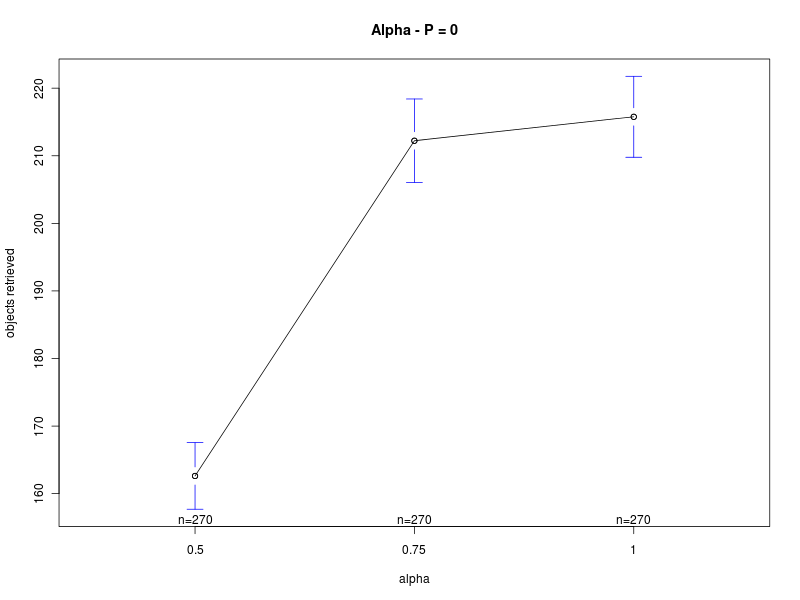
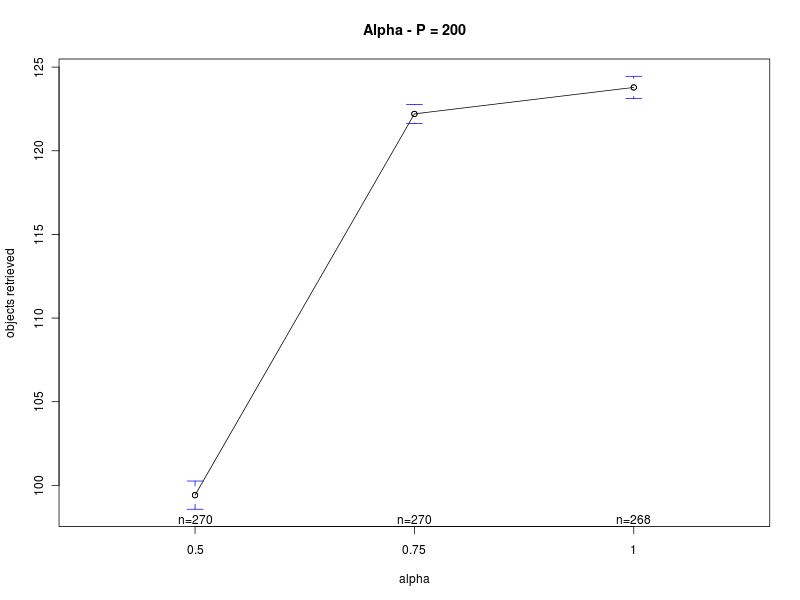
- Weighted average factor alpha: 0.5, 0.75, 1.0
For the results of the four ANOVAs please refer to:
- ANOVA - including the interfacing time Π as factor
- ANOVA - interfacing time Π = 0 s
- ANOVA - interfacing time Π = 100 s
- ANOVA - interfacing time Π = 200 s
Summary of the results
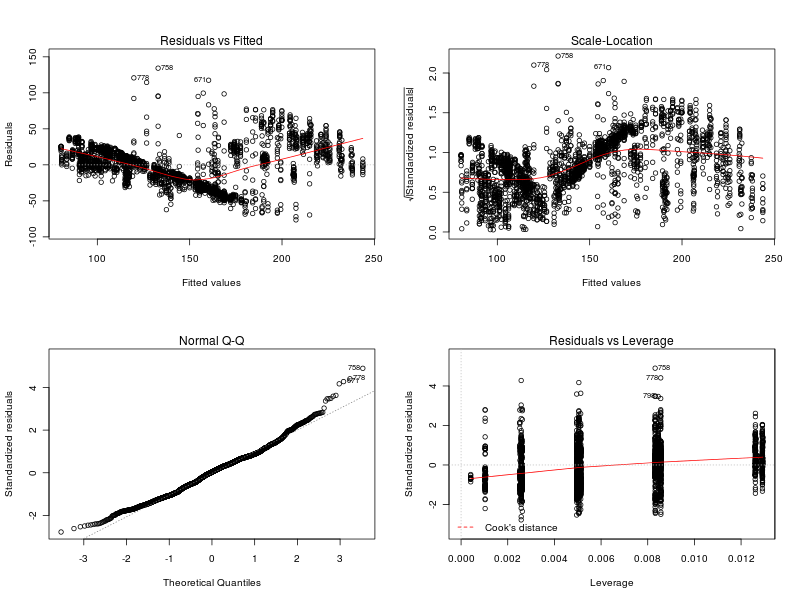
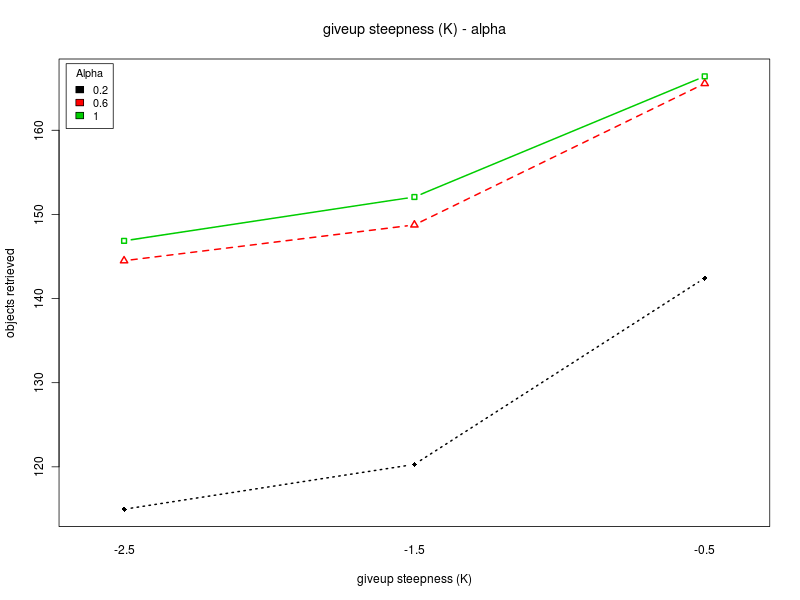
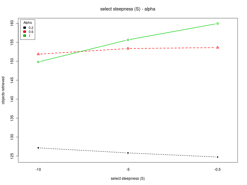
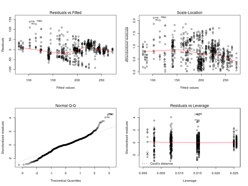
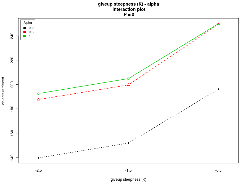
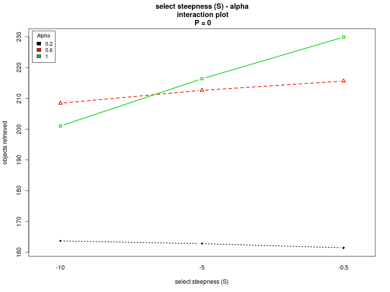
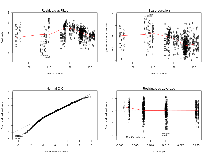
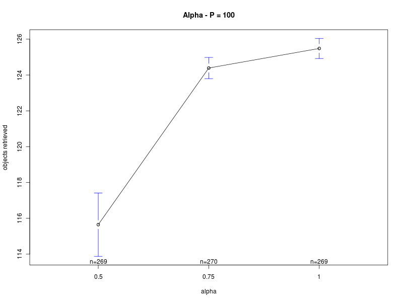
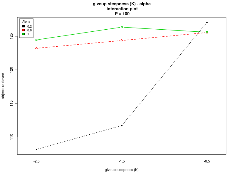
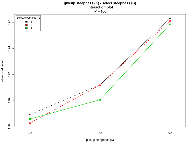
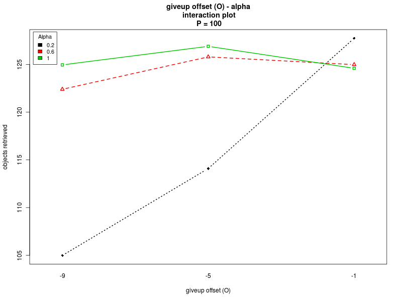
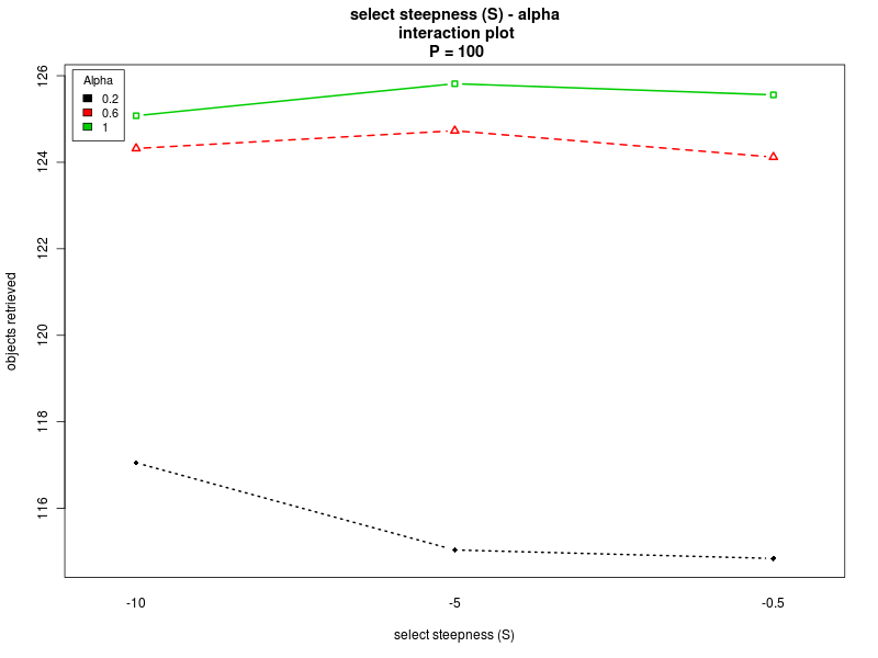
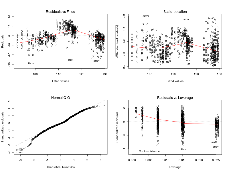
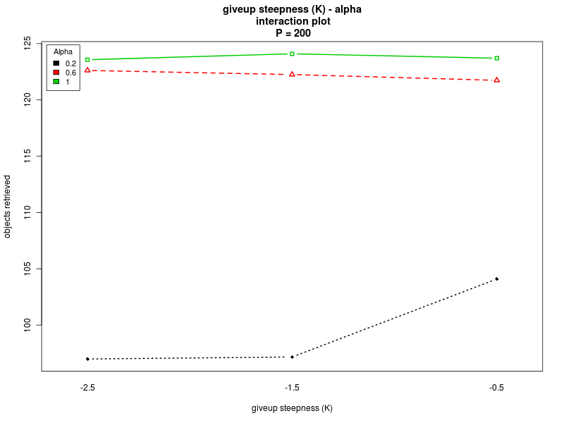
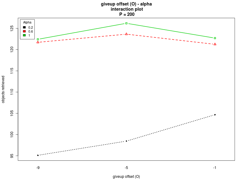
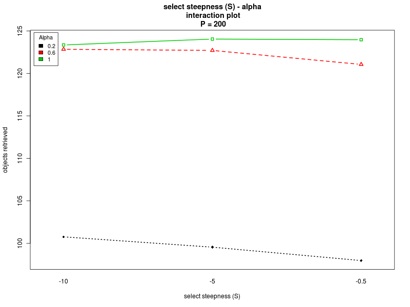
This section summarizes the results obtained with the four analyses. The results show that there are normality violations in the data (see plots: analysis including Π as factor, for Π=0, for Π=100, and for Π=200). Nevertheless, most of the data is normally distributed, and this allows us to analyise the main trends.Concerning the parameter alpha, the four analyses suggest that a high value of the parameter is preferable. Both the main effect plots and the interaction plots show that high values of alpha are related to an increse in the performance. The fact that low values of alpha impact negatively on the performance suggests that when alpha is too low the robot are not able to quickly evaluate the current environmental conditions and choose a proper strategy accordingly. Alpha is in fact used when computing the weighted averages, with lower values of alpha giving less importance to the last measured value.
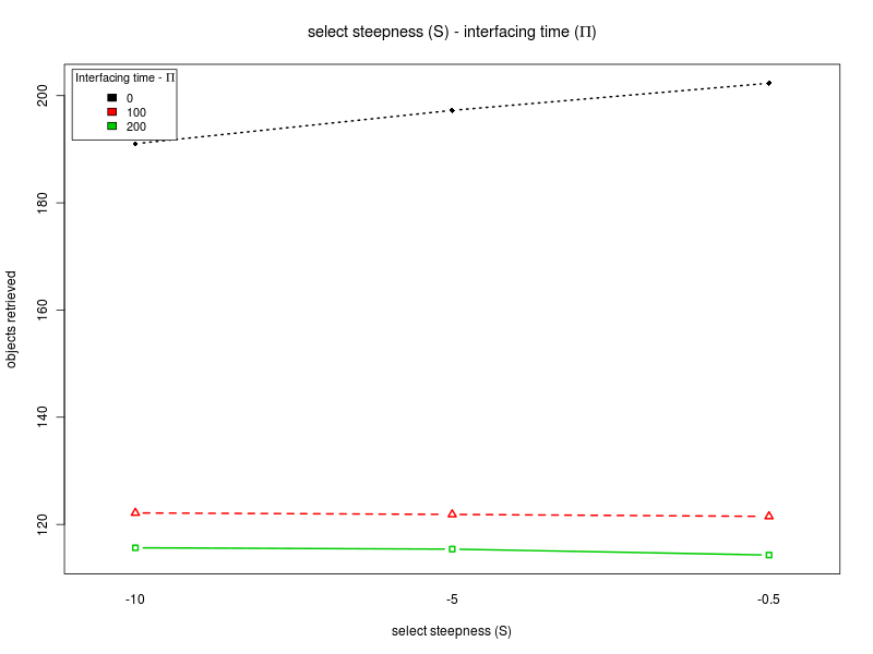
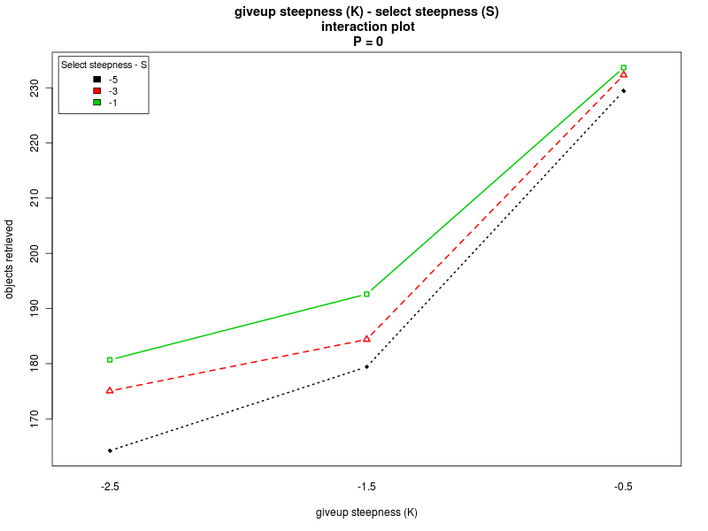
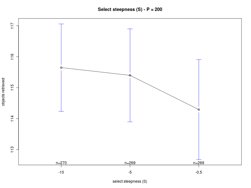
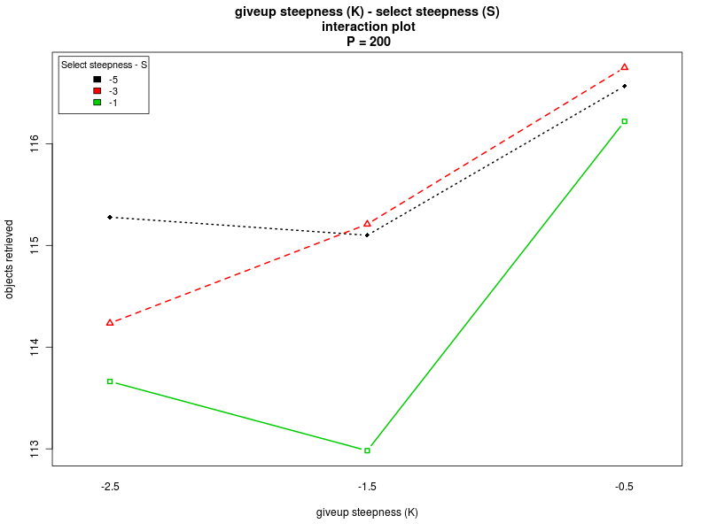
Concerning the parameter S, the main effects plot for the first analysis suggests that the parameter does not have a big impact on the performance. However, the result is probably due to the fact that the effects of the parameter change with the value of Π (see interaction plot and main effect plots for Π = 0 and Π = 200). In fact, for low values of the interfacing time Π, a high value of S is preferable. Conversely, when Π is high, lower values of S should be chosen. Therefore, to properly select the value for the parameter, one should take into account the specific situation. If the value of the interfacing time Π is known or can be roughly estimated, and it is known that it does not change over time, then S can be selected accordingly. In the case in which the value of Π is not known, or it may change it time, then an intermediate value for S should be chosen.
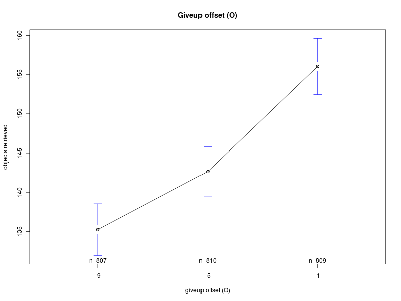
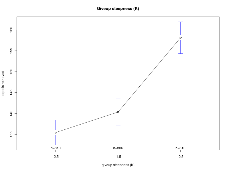
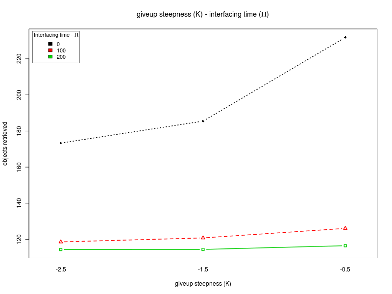
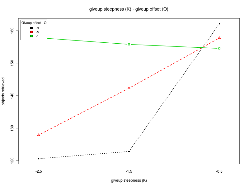
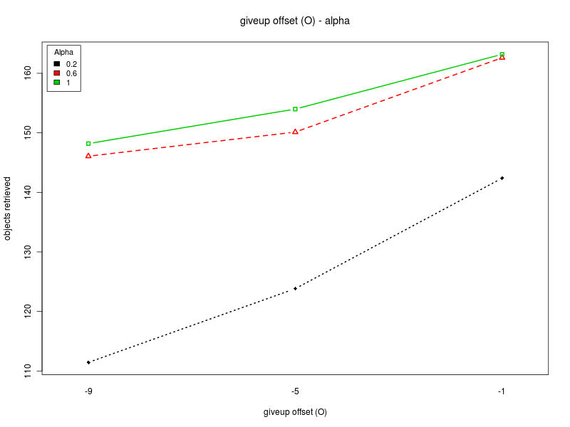
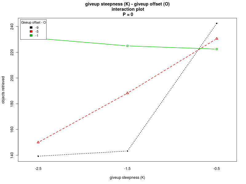
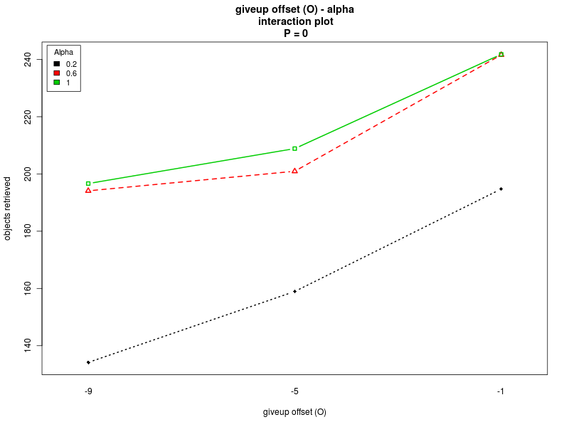
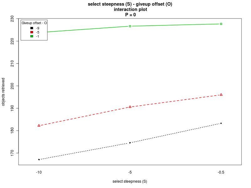
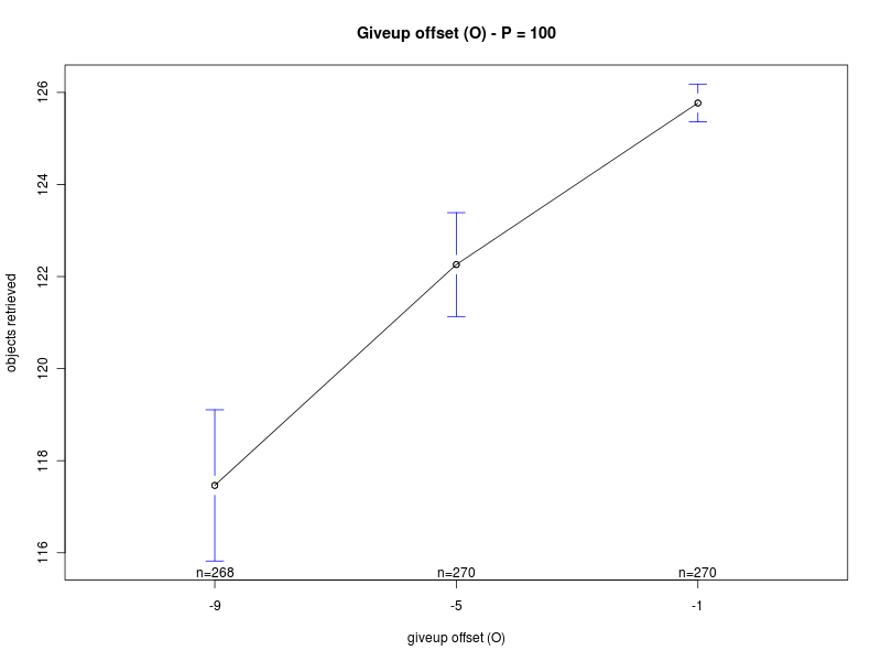
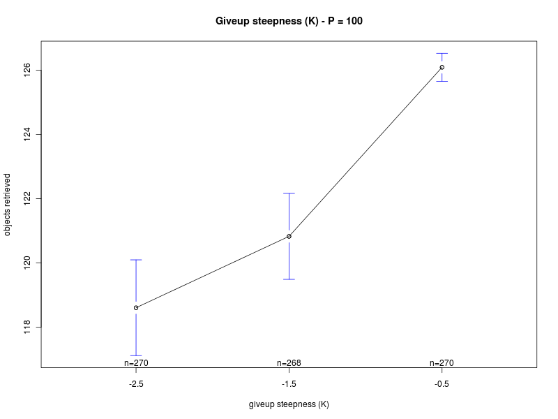
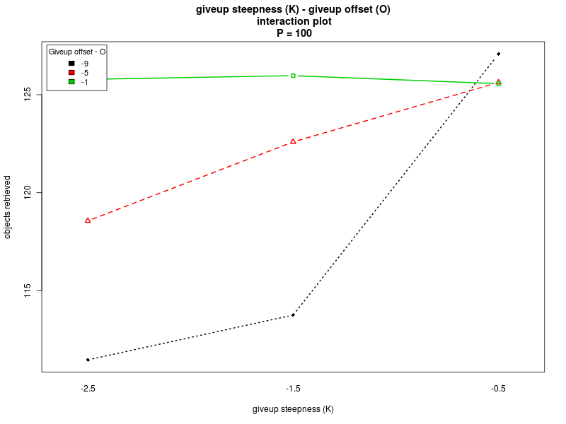
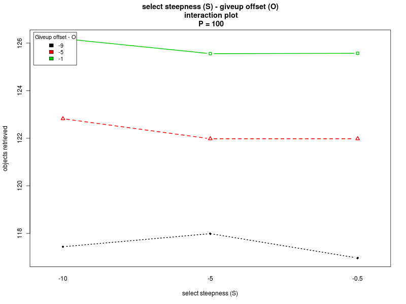
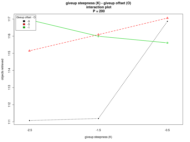
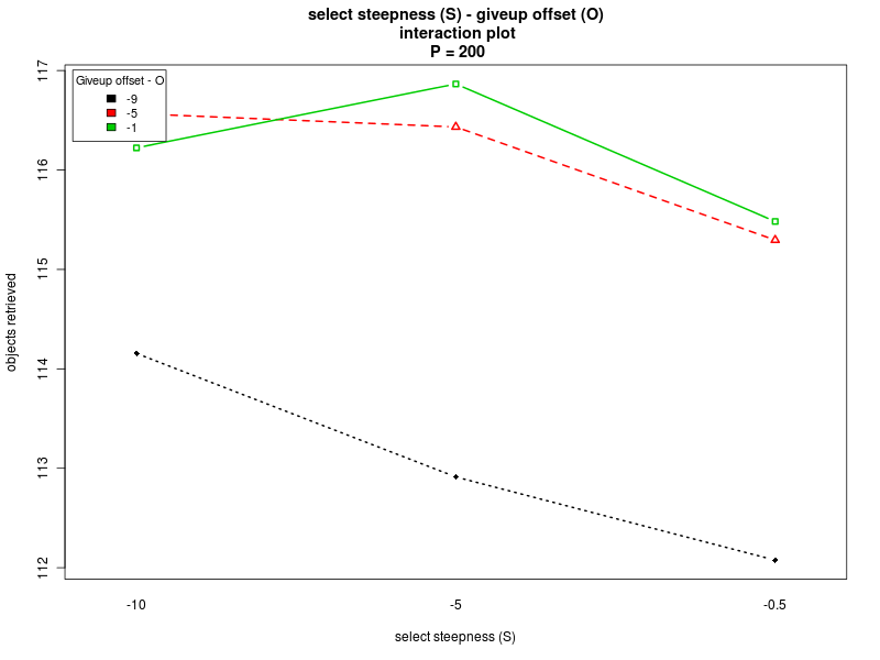
Concerning K and O, the interaction plots show that there is a strong interaction between the values of K and O, for all the values of Π. Their effect is highly variable, depending on their combination and the value of Π (see plots: analysis including Π as factor, for Π = 0, and for Π = 200). A deeper analysis, on the interactions of orders higher than the second, could help having a better understanding on how the two parameters should be chosen. Nevertheless it seems that a combination with high values for both the parameters is preferable.
Top
ANOVA - including the interfacing time Π as factor
This section is about the ANOVA for the case in which Π is treated as a factor. In the following you can find:- Summary of the analysis (R output) and graphs to verify the ANOVA assumptions.
- Main effects plots for each of the factors
- Interaction plots between the factors
                                 Df  Sum Sq Mean Sq   F value    Pr(>F)
steepness K                       1  208615  208615  275.6000 < 2.2e-16 ***
offset O                          1  175151  175151  231.3904 < 2.2e-16 ***
alpha                             1  345106  345106  455.9172 < 2.2e-16 ***
steepness S                       1    4025    4025    5.3176 0.0211961 *
interfacing time Π             1 2703103 2703103 3571.0477 < 2.2e-16 ***
steepness K:offset O              1  135592  135592  179.1291 < 2.2e-16 ***
steepness K:alpha                 1    4238    4238    5.5988 0.0180517 *
steepness K:steepness S           1     926     926    1.2233 0.2688299
steepness K:interfacing time Π 1  214450  214450  283.3079 < 2.2e-16 ***
offset O:alpha                    1   17133   17133   22.6340 2.076e-06 ***
offset O:steepness S              1     929     929    1.2278 0.2679377
offset O:interfacing time Π    1  155290  155290  205.1530 < 2.2e-16 ***
alpha:steepness S                 1   10447   10447   13.8020 0.0002077 ***
alpha:interfacing time Π       1   56067   56067   74.0698 < 2.2e-16 ***
steepness S:interfacing time Π 1   10746   10746   14.1960 0.0001687 ***
Residuals                      2410 1824248     757

Signif. codes:  0 '***' 0.001 '**' 0.01 '*' 0.05 '.' 0.1 ' ' 1
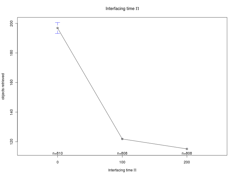
Main effects plots
Click on a plot to enlarge it.| Alpha | Steepness S |
 |
 |
| Offset O | Steepness K |
 |
 |
| Interfacing time Π | |
 |
| Anova index | Top |
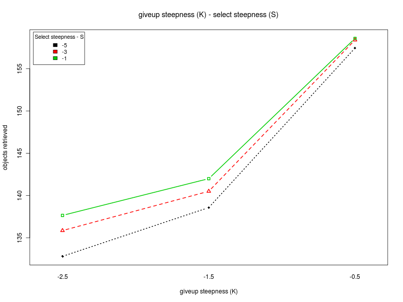
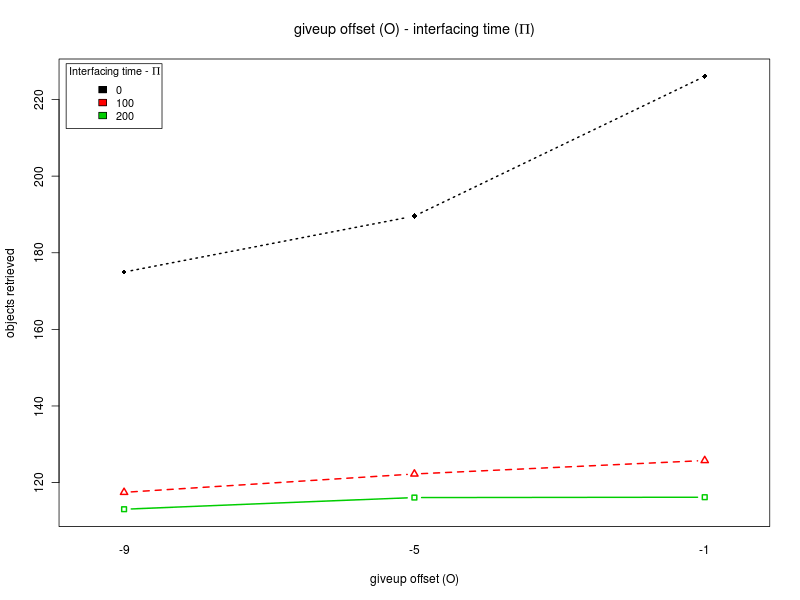
Interaction plots
Click on a plot to enlarge it.| Steepness K - interfacing time Π | Steepness K - alpha |
 |
 |
| Steepness K - Offset O | Steepness K - Steepness S |
 |
 |
| Offset O - interfacing time Π | Offset O - Alpha |
 |
 |
| Steepness S - interfacing time Π | Steepness S - Alpha |
 |
 |
| Alpha - interfacing time Π | 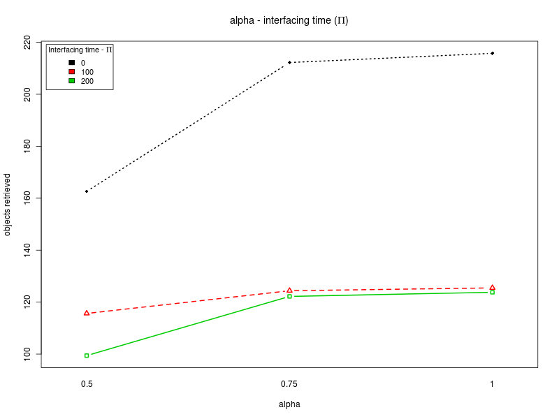 |
| Anova index | Top |
ANOVA - interfacing time Π = 0
This section is about the ANOVA for the case in which Π is not treated as a factor and is set to 0. In the following you can find:- Summary of the analysis (R output) and graphs to verify the ANOVA assumptions.
- Main effects plots for each of the factors
- Interaction plots between the factors
                         Df  Sum Sq Mean Sq  F value    Pr(>F)
steepness K               1 461770  461770 465.9464 < 2.2e-16 ***
offset O                  1 352268  352268 355.4543 < 2.2e-16 ***
alpha                     1 381264  381264 384.7120 < 2.2e-16 ***
steepness S               1  17237   17237  17.3927 3.373e-05 ***
steepness K:offset O      1 279714  279714 282.2444 < 2.2e-16 ***
steepness K:alpha         1     23      23   0.0232   0.87895
steepness K:steepness S   1   3403    3403   3.4339   0.06424 .
offset O:alpha            1   5358    5358   5.4061   0.02032 *
offset O:steepness S      1   3407    3407   3.4376   0.06410 .
alpha:steepness S         1  21781   21781  21.9780 3.242e-06 ***
Residuals               799 791838     991

Signif. codes:  0 '***' 0.001 '**' 0.01 '*' 0.05 '.' 0.1 ' ' 1
Main effects plots (D=0)
Click on a plot to enlarge it.| Alpha | Offset O |
 |
 |
| Steepness K | Steepness S |
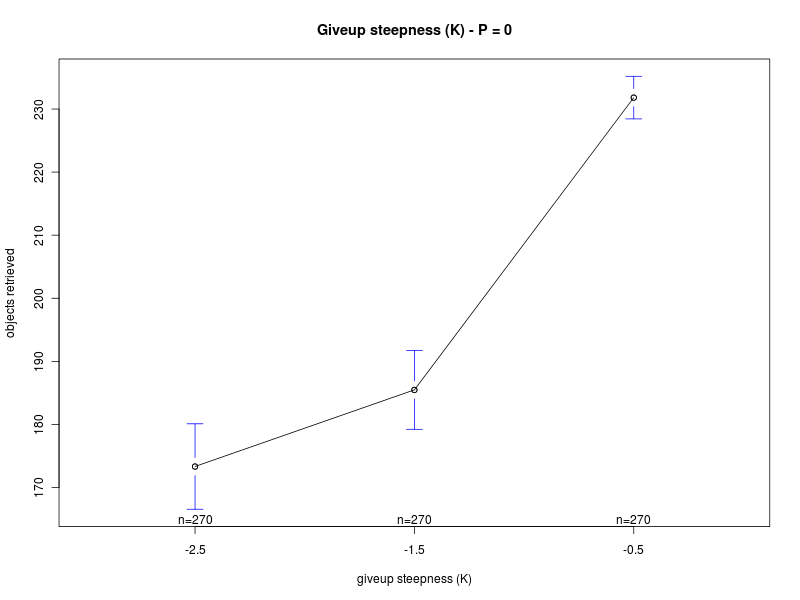 |
 |
| Anova - Π = 0 - index | Top |
Interaction plots (Π=0)
Click on a plot to enlarge it.| Steepness K - Alpha | Steepness K - Offset O |
 |
 |
| Steepness K - Steepness S | Offset O - Alpha |
 |
 |
| Steepness S - Alpha | Steepness S - Offset O |
 |
 |
| Anova - Π = 0 - index | Top |
ANOVA - interfacing time Π = 100
This section is about the ANOVA for the case in which Π is not treated as a factor and is set to 100. In the following you can find:- Summary of the analysis (R output) and graphs to verify the ANOVA assumptions.
- Main effects plots for each of the factors
- Interaction plots between the factors
                         Df Sum Sq Mean Sq   F value    Pr(>F)
steepness K               1  7557.8  7557.8 192.1798 < 2e-16 ***
offset O                  1  9275.9  9275.9 235.8673 < 2e-16 ***
alpha                     1 13009.7 13009.7 330.8102 < 2e-16 ***
steepness S               1    55.7    55.7   1.4159 0.23444
steepness K:offset O      1  5635.9  5635.9 143.3092 < 2e-16 ***
steepness K:alpha         1  7137.8  7137.8 181.5003 < 2e-16 ***
steepness K:steepness S   1     0.2     0.2   0.0059 0.93856
offset O:alpha            1 11962.7 11962.7 304.1882 < 2e-16 ***
offset O:steepness S      1     0.7     0.7   0.0183 0.89257
alpha:steepness S         1   169.6   169.6   4.3131 0.03814 *
Residuals               797 31343.4    39.3

Signif. codes:  0 '***' 0.001 '**' 0.01 '*' 0.05 '.' 0.1 ' ' 1
Main effects plots (Π=100)
Click on a plot to enlarge it.| Alpha | Offset O |
 |
 |
| Steepness K | Steepness S |
 |
 |
| Anova - Π = 100 - index | Top |
Interaction plots (Π=100)
Click on a plot to enlarge it.| Steepness K - Alpha | Steepness K - Offset O |
 |
 |
| Steepness K - Steepness S | Offset O - Alpha |
 |
 |
| Steepness S - Alpha | Steepness S - Offset O |
 |
 |
| Anova - Π = 100 - index | Top |
ANOVA - interfacing time Π = 200
This section is about the ANOVA for the case in which Π is not treated as a factor and is set to 200. In the following you can find:- Summary of the analysis (R output) and graphs to verify the ANOVA assumptions.
- Main effects plots for each of the factors
- Interaction plots between the factors
                         Df Sum Sq Mean Sq   F value    Pr(>F)
steepness K               1    607     607   11.7743 0.0006315 ***
offset O                  1   1322    1322   25.6576 5.069e-07 ***
alpha                     1  80043   80043 1553.2974 < 2.2e-16 ***
steepness S               1    227     227    4.4086 0.0360725 *
steepness K:offset O      1   1145    1145   22.2176 2.873e-06 ***
steepness K:alpha         1   1093    1093   21.2186 4.769e-06 ***
steepness K:steepness S   1     37      37    0.7255 0.3946134
offset O:alpha            1   1932    1932   37.4919 1.440e-09 ***
offset O:steepness S      1     33      33    0.6484 0.4209138
alpha:steepness S         1    269     269    5.2247 0.0225304 *
Residuals               797  41070      52

Signif. codes:  0 '***' 0.001 '**' 0.01 '*' 0.05 '.' 0.1 ' ' 1
Main effects plots (Π=200)
Click on a plot to enlarge it.| Alpha | Offset O |
 |
 |
| Steepness K | Steepness S |
 |
 |
| Anova - Π = 200 - index | Top |
Interaction plots (Π=200)
Click on a plot to enlarge it.| Steepness K - Alpha | Steepness K - Offset O |
 |
 |
| Steepness K - Steepness S | Offset O - Alpha |
 |
 |
| Steepness S - Alpha | Steepness S - Offset O |
 |
 |
| Anova - Π = 200 - index | Top |